Modeling psychological impacts on epidemic spread: the effect of vacationers on a network
Modeling the effect of outside travellers on epidemic spread in an agent-based simulation
This model is based on the model/simulation found found here.
The agent
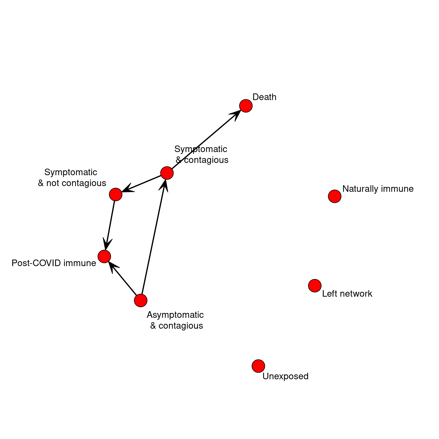
We will augment the agent with an additional state–not in network. This will let us have ‘vacationer’ or ‘traveller’ agents that leave the network and no longer impact anyone.
- Unexposed
- Asymptomatic but infected/contagious
- Symptomatic and contagious
- Symptomatic and not contagious
- Post-COVID Immune
- Naturally immune (will not contract)
- Death
- Left network
##
## Attaching package: 'dplyr'
## The following objects are masked from 'package:stats':
##
## filter, lag## The following objects are masked from 'package:base':
##
## intersect, setdiff, setequal, union## Loading required package: statnet.common##
## Attaching package: 'statnet.common'## The following object is masked from 'package:base':
##
## order## Loading required package: network## network: Classes for Relational Data
## Version 1.16.0 created on 2019-11-30.
## copyright (c) 2005, Carter T. Butts, University of California-Irvine
## Mark S. Handcock, University of California -- Los Angeles
## David R. Hunter, Penn State University
## Martina Morris, University of Washington
## Skye Bender-deMoll, University of Washington
## For citation information, type citation("network").
## Type help("network-package") to get started.## sna: Tools for Social Network Analysis
## Version 2.5 created on 2019-12-09.
## copyright (c) 2005, Carter T. Butts, University of California-Irvine
## For citation information, type citation("sna").
## Type help(package="sna") to get started.##
## Attaching package: 'igraph'## The following objects are masked from 'package:sna':
##
## betweenness, bonpow, closeness, components, degree, dyad.census,
## evcent, hierarchy, is.connected, neighborhood, triad.census## The following objects are masked from 'package:network':
##
## %c%, %s%, add.edges, add.vertices, delete.edges, delete.vertices,
## get.edge.attribute, get.edges, get.vertex.attribute, is.bipartite,
## is.directed, list.edge.attributes, list.vertex.attributes,
## set.edge.attribute, set.vertex.attribute## The following objects are masked from 'package:dplyr':
##
## as_data_frame, groups, union## The following objects are masked from 'package:stats':
##
## decompose, spectrum## The following object is masked from 'package:base':
##
## union## Registered S3 method overwritten by 'GGally':
## method from
## +.gg ggplot2##
## Attaching package: 'GGally'## The following object is masked from 'package:dplyr':
##
## nasalibrary(rlist)
#library(animation)
STATES <<- 8
STATENAMES <<- c("Unexposed",
"Asymptomatic & contagious",
"Symptomatic and contagious",
"Symptomatic and not contagious",
"Post-COVID immune",
"Naturally immune",
"Death",
"Left")
STATELABELS <<- c("Unexposed","Asymptomatic\n & contagious",
"Symptomatic \n& contagious",
"Symptomatic \n& not contagious",
"Post-COVID immune",
"Naturally immune",
"Death",
"Left network")Create transition matrix.
makeAgent <- function(psychstate,biostate,age=30,traveler=0,is_infected = 0)
{

  return (list(psychstate=psychstate,
               biostate=biostate,
               age=age,
               nextbiostate=NA,
               biostatecountdown=NA,traveler=traveler,is_infected = is_infected))
}

# * 1. Unexposed
# * 2. Asymptomatic but infected/contagious
# * 3. Symptomatic and contagious
# * 4. Symptomatic and not contagious
# * 5. Post-COVID Immune
# * 6. Naturally immune (will not contract)
# * 7. Death
# * 8. Left network


bioTransition <- matrix(0,STATES,STATES)
bioMin <- matrix(1,STATES)      #state time minimum
bioMax <- matrix(1,STATES)      #state time maximum


bioMin[2] <- 3            #infected but asymptomatic for 3 to 10 days
bioMax[2] <- 10
bioTransition[2,3] <- .1  #transition to infected with symptoms
bioTransition[2,5] <- .90  #transition to no longer contagious/cured


bioMin[3] <-    3             #symptoms + contagion
bioMax[3] <- 8                #symptoms + contagion max
bioTransition[3,4] <-  .95    #transitioon to no longer contagious
bioTransition[3,7] <-  .05    #transitioon to death state


bioMin[4] <- 1          #symptoms bot no longer contagiious
bioMax[4] <- 7
bioTransition[4,5] <- 1  #Transition to 'immune' cured state.


setAgentState<- function(agent, biostate)
{
  agent$biostate <- biostate
  if(sum(bioTransition[biostate,])>0) # this state transitions to something else.
  {
    ##which state do we go to?
     agent$biostatecountdown <- sample(x=seq(bioMin[biostate],bioMax[biostate]),1) #how long will we state in this state?
     agent$nextbiostate <- sample(1:STATES, prob=bioTransition[agent$biostate,],size=1)

  } else{
   agent$biostatecountdown <- NA
   agent$nextbiostate <- NA   ##just so we can tell if the agent is finished.
  }
  return(agent)
}

transitionAgent<- function(agent)
{
   return(setAgentState(agent,agent$nextbiostate))
}

updateAgent<- function(agent)
{
  if(!is.na(agent$biostatecountdown))
  {
   agent$biostatecountdown <- agent$biostatecountdown -1
    if(agent$biostatecountdown <=0)  ##new state
    {
       agent <- transitionAgent(agent)

    }
  }
   return(agent)
}

setAgentStatusInfected<- function(agent,status=1)
{
   agent$is_infected <- status
   return(agent)
}
Adding a new agent to the network
Here, we write code that will grow the network by adding new agents.
addAgentToNetwork<- function(numAgents=5,prev_network = socialnetwork,connection_number=1,self_connected=1,pool)
{

   if(connection_number < 1){

     connection_number <- 1
   }

   number_of_rows <- nrow(prev_network)

   starting_point <- number_of_rows+1
   end_point <- number_of_rows + numAgents


    for(i in starting_point:end_point) {

      prev_network <- rbind(prev_network, 0)
      prev_network <- cbind(prev_network, 0)


    }


  if(number_of_rows>= connection_number ){

    #x <- 1:number_of_rows

    u <- 1:number_of_rows

    for (val in u) {

      if((pool[[val]]$biostate != 8) ){

        if((pool[[val]]$biostate != 7)){
          x<-u
        }
      }

    }


     a <- sample(x, connection_number)
     # print("SSSSSSSSSSSSSSSSSSSS")
     # print(a)
     #


    # repeat{
    #
    #   if((pool[[a]]$biostate != 8) ){
    #
    #     if((pool[[a]]$biostate != 7)){
    #       break
    #     }
    #
    #   }
    # }
   # print(a)


     for(i in starting_point:end_point) {
          if(self_connected==1){

             prev_network[i,i] <- 1
          }

        current_new_agent <-i
        for (i in seq_along(a)) {

          #print(a[i])
          prev_network[a[i],current_new_agent] <- 1
          prev_network[current_new_agent,a[i]] <- 1
        }


    }


  }
   else{

     #x <- 1:number_of_rows
     # print("SSSSSSSSSggfgfgSSSSSSSSSSS")
     # print(a)
     #
    u <- 1:number_of_rows

    for (val in u) {

      if((pool[[val]]$biostate != 8) ){

        if((pool[[val]]$biostate != 7)){
          x<-u
        }
      }

    }

     a <- sample(x, 1)


   # print(a)


     for(i in starting_point:end_point) {
          if(self_connected==1){

             prev_network[i,i] <- 1
          }

        current_new_agent <-i
        for (i in seq_along(a)) {

          #print(a[i])
          prev_network[a[i],current_new_agent] <- 1
          prev_network[current_new_agent,a[i]] <- 1
        }


    }


   }


  return(prev_network)


}
Background
A key step in contingency planning for a possible pandemic in a community is barring entry of travelers in the community. The potential for infectious diseases to spread in a community rapidly through well-connected infected travelers in the community is very high. Past researches looked into the effect of the international travel ban on reducing the spread of disease in countries. Partial restriction of travel helps in slowing the spread if the global number of cases of infection is low (Hollingsworth et al., 2006). According to Epstein et al. (2007), international air travel restrictions may provide a small but important delay in the spread of a pandemic, especially if other disease control measures are implemented during a timeframe. Using the mathematical model, Cooper et al. (2006) concluded that restrictions on air travel would achieve very little. This is probably because a virus may transmit from one person to another very quickly and affects many people. Once a major outbreak is underway, banning flights from affected cities would be effective at significantly delaying spread only if almost all travel between cities could be stopped almost as soon as an outbreak was detected in each city.
One of the main reasons against oversea travel ban is because it has a big negative economic impact in a country if we stop adults traveling oversea (Lam et al., 2011). But for small and moderate length communities whose economic activities circulated within the community, a travel restriction may be helpful during a pandemic. If the health care systems for these communities are not prepared to deal with a pandemic, it is better to enforce some sort of travel ban so that the health care system does not overwhelm with patients. This will help to keep a check on the number of patients. In the traditional SIR model (Smith & Moore, 2004), it is not defined how adding travelers to the scenario will affect the spread of disease. So, we created an agent-based social model for a community where we will be adding travelers to the local populations to see how a disease spreads in the whole community. We will be looking into the worst-case scenario in the model, where travelers will enter the community but nobody leaves within a timeframe from the community. We will vary different variables in the simulations to see the disease progress in the community within a specific timeframe.
References
- Cooper, B. S., Pitman, R. J., Edmunds, W. J., & Gay, N. J. (2006). Delaying the international spread of pandemic influenza. PLoS Medicine, 3(6).
- Epstein, J. M., Goedecke, D. M., Yu, F., Morris, R. J., Wagener, D. K., & Bobashev, G. V. (2007). Controlling pandemic flu: The value of international air travel restrictions. PloS One, 2(5).
- Hollingsworth, T. D., Ferguson, N. M., & Anderson, R. M. (2006). Will travel restrictions control the international spread of pandemic influenza? Nature Medicine, 12(5), 497–499.
- Lam, E. H., Cowling, B. J., Cook, A. R., Wong, J. Y., Lau, M. S., & Nishiura, H. (2011). The feasibility of age-specific travel restrictions during influenza pandemics. Theoretical Biology and Medical Modelling, 8(1), 44.
- Smith, D., & Moore, L. (2004). The SIR Model for Spread of Disease: The Differential Equation Model. Loci.(Originally Convergence.) Https://Www. Maa. Org/Press/Periodicals/Loci/Joma/the-Sir-Model-for-Spread-of-Disease-the-Differential-Equation-Model.
Travel ban lift and allowing traveler to the community
Initial simulation
For this first simulation, No locals are affected with a strain from beginning.
  numAgents_initial <<- 700
  naturalImmunity <- .01
  socialnetwork <-makeNetwork(numAgents_initial,numsets=1,power=.5,steps=2)
  local_population_infection_number <-0

  infect_local <- 0

  original_network_of_agents <<- socialnetwork

  .GlobalEnv$pool <- list()
  for(i in 1:numAgents_initial)
  {
     .GlobalEnv$pool[[i]] <- makeAgent(psychstate=1,
                           biostate=sample(c(1,6),
                            p=c(1-naturalImmunity, naturalImmunity),1))
  }

  ##infect patient 0
  numInfected <- 3
  for(i in sample(numAgents_initial,numInfected))
  {
    if(infect_local){

       .GlobalEnv$pool[[i]] <- setAgentState(pool[[i]],2) ##infect this person


       if(.GlobalEnv$pool[[i]]["biostate"] == 2){
         if(.GlobalEnv$pool[[i]]["is_infected"] == 0){
           local_population_infection_number <-local_population_infection_number+1
          .GlobalEnv$pool[[i]] <- setAgentStatusInfected( .GlobalEnv$pool[[i]],1)
         }

       }
    }

  }

  pool_initial <<-.GlobalEnv$pool
  local_population_infection_number <<- local_population_infection_number
Travel ban
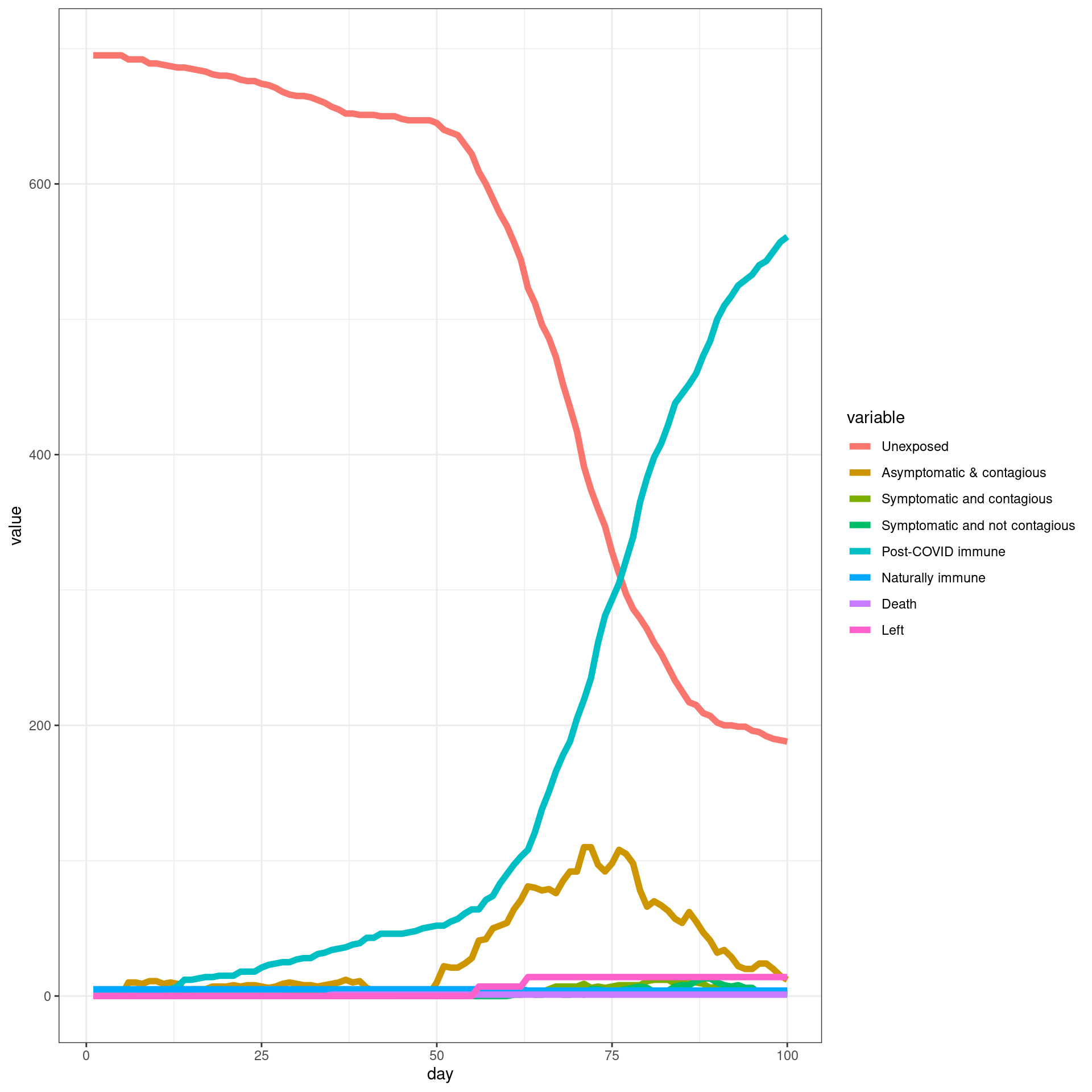
In this simulation, a ‘travel ban’ is implemented from Day 7 and removed early (In this case from day 49). Each traveler will have only three connections with local agents. For this simulation, we will look at the spread of the disease through the network over time.
  numDays = 100
  enable_outside_travel_restriction_day <- 7
  second_wave_day <- as.integer((49/100)*numDays)
    #

  #as.integer((numAgents_initial)*(1/100))
  disthistory <- travel_ban_lift(enable_outside_travel_restriction_day,second_wave_day,
                  connection_number = 3,will_affect_traveler = 1,numDays = numDays  )
## [1] "TOTAL"
## [1] 791
## [1] "Total Local"
## [1] 700
## [1] "Local Death"
## [1] 4
## [1] "-----"
## [1] "Total Traveler"
## [1] 91
## [1] "Traveler Death"
## [1] 0
## [1] "Local infected at somepoint"
## [1] 536
## [1] "Traveler infected at somepoint"
## [1] 84
## [1] "Total infected at somepoint"
## [1] 620 disthist.df <-as.data.frame(disthistory)
colnames(disthist.df) <- STATENAMES
disthist.df$day <- 1:nrow(disthistory)
histlong <- melt(disthist.df,id.vars="day")
ggplot(histlong,aes(x=day,y=value,fill=variable)) + geom_bar(stat="identity",position="stack") +
theme_bw() ##make the SIR plot:
sir <- data.frame(day=disthist.df$day,
susceptible = disthist.df$Unexposed,
infected = disthist.df[,2]+disthist.df[,3],
recovered = rowSums(disthist.df[,4:7]))
ggplot(melt(sir,id.vars="day"),aes(x=day,group=variable,y=value,color=variable)) + geom_line(size=2) + theme_bw()
Travel ban/early removal
In this simulation, a ban is implemented from Day 7 and removed early (In this case from day 49). Each traveler will have only one connection with local agents
numDays = 100
enable_outside_travel_restriction_day <- 7
second_wave_day <- as.integer((49/100)*numDays)
#as.integer((numAgents_initial)*(1/100))
disthistory <- travel_ban_lift(enable_outside_travel_restriction_day,second_wave_day,
connection_number = 1,will_affect_traveler = 1,numDays = numDays ) 
## [1] "TOTAL"
## [1] 791
## [1] "Total Local"
## [1] 700
## [1] "Local Death"
## [1] 1
## [1] "-----"
## [1] "Total Traveler"
## [1] 91
## [1] "Traveler Death"
## [1] 0
## [1] "Local infected at somepoint"
## [1] 497
## [1] "Traveler infected at somepoint"
## [1] 84
## [1] "Total infected at somepoint"
## [1] 581 disthist.df <-as.data.frame(disthistory)
colnames(disthist.df) <- STATENAMES
disthist.df$day <- 1:nrow(disthistory)
histlong <- melt(disthist.df,id.vars="day")
ggplot(histlong,aes(x=day,y=value,fill=variable)) + geom_bar(stat="identity",position="stack") +
theme_bw()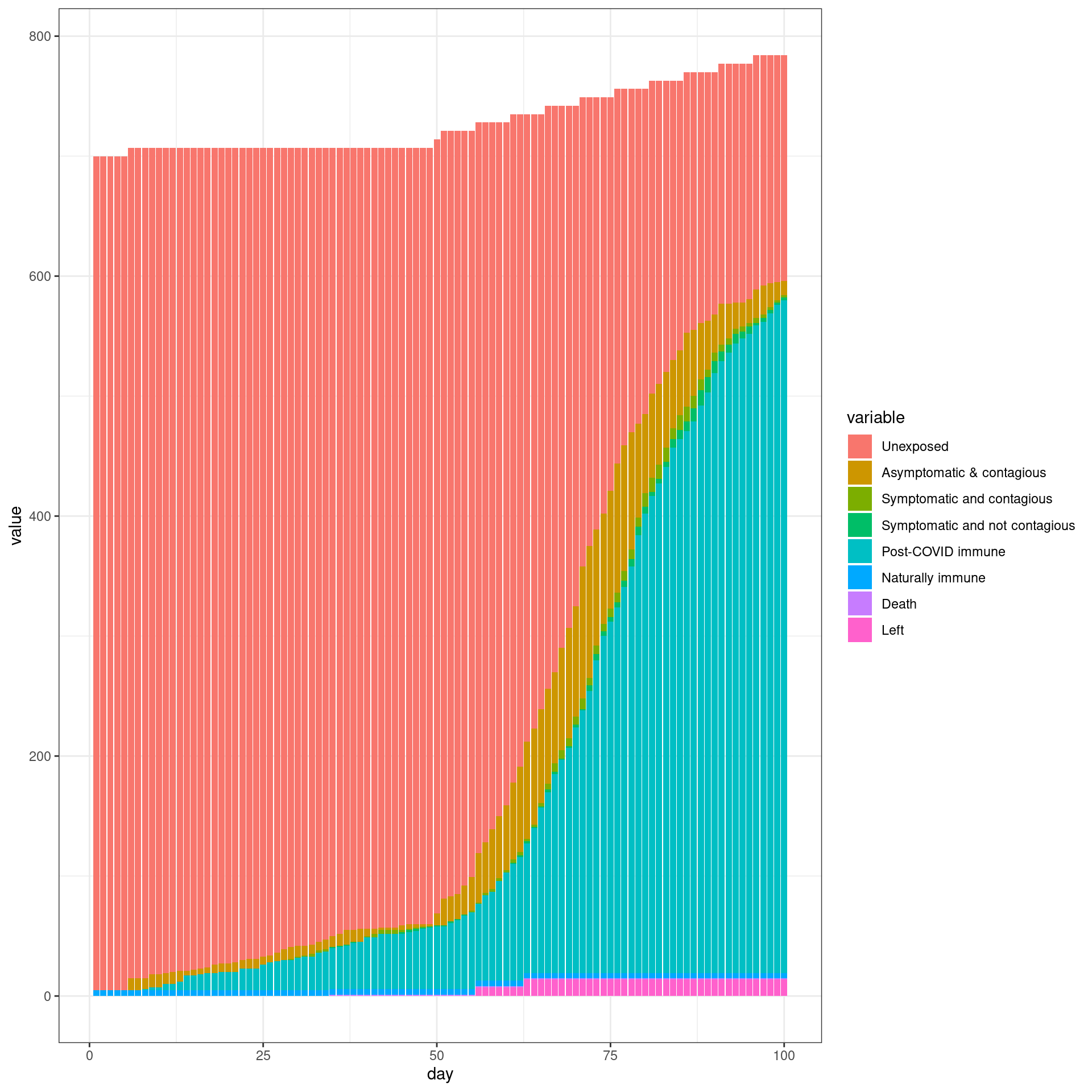
  ##make the SIR plot:
  sir <- data.frame(day=disthist.df$day,
                    susceptible = disthist.df$Unexposed,
                    infected = disthist.df[,2]+disthist.df[,3],
                    recovered = rowSums(disthist.df[,4:7]))

  ggplot(melt(sir,id.vars="day"),aes(x=day,group=variable,y=value,color=variable)) + geom_line(size=2) + theme_bw()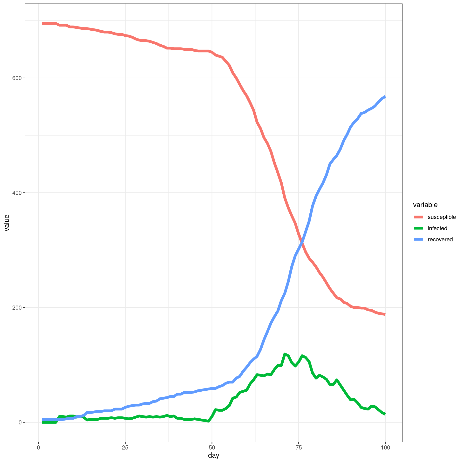
Travel ban/late removal
In this simulation, a ban is implemented from Day 7 and removed later (In this case from day 80). Each traveler will have only three connection with local agents
# numDays = 250
# enable_outside_travel_restriction_day <- 7
# second_wave_day <- as.integer((80/100)*numDays)
#
# #as.integer((numAgents_initial)*(1/100))
# disthistory <- travel_ban_lift(enable_outside_travel_restriction_day,second_wave_day,
# connection_number = 3,will_affect_traveler = 1,numDays = numDays )
#
# disthist.df <-as.data.frame(disthistory)
# colnames(disthist.df) <- STATENAMES
# disthist.df$day <- 1:nrow(disthistory)
# histlong <- melt(disthist.df,id.vars="day")
#
# ggplot(histlong,aes(x=day,y=value,fill=variable)) + geom_bar(stat="identity",position="stack") +
# theme_bw()
#
# ##make the SIR plot:
# sir <- data.frame(day=disthist.df$day,
# susceptible = disthist.df$Unexposed,
# infected = disthist.df[,2]+disthist.df[,3],
# recovered = rowSums(disthist.df[,4:7]))
#
# ggplot(melt(sir,id.vars="day"),aes(x=day,group=variable,y=value,color=variable)) + geom_line(size = 2) + theme_bw()
# ggplot(histlong,aes(x=day,y=value,group=variable,color=variable)) + geom_line(size = 2) + theme_bw()Second simulation series
In this series of simulations, some locals are affected with a strain from beginning, and travellers will augment this by bringing the disease in from outside.
numAgents_initial <<- 700
naturalImmunity <- .01
socialnetwork <-makeNetwork(numAgents_initial,numsets=1,power=.5,steps=2)
local_population_infection_number <-0
infect_local <- 1
original_network_of_agents <<- socialnetwork
.GlobalEnv$pool <- list()
for(i in 1:numAgents_initial)
{
.GlobalEnv$pool[[i]] <- makeAgent(psychstate=1,
biostate=sample(c(1,6),
p=c(1-naturalImmunity, naturalImmunity),1))
}
##infect patient 0
numInfected <- 3
for(i in sample(numAgents_initial,numInfected))
{
if(infect_local){
.GlobalEnv$pool[[i]] <- setAgentState(pool[[i]],2) ##infect this person
if(.GlobalEnv$pool[[i]]["biostate"] == 2){
if(.GlobalEnv$pool[[i]]["is_infected"] == 0){
local_population_infection_number <-local_population_infection_number+1
.GlobalEnv$pool[[i]] <- setAgentStatusInfected( .GlobalEnv$pool[[i]],1)
}
}
}
}
pool_initial <<-.GlobalEnv$pool
local_population_infection_number <<- local_population_infection_numberIF no traveler is allowed and some locals are infected
# numDays = 100
# enable_outside_travel_restriction_day <- 1
# second_wave_day <- 101
#
# #as.integer((numAgents_initial)*(1/100))
# disthistory <- travel_ban_lift(enable_outside_travel_restriction_day,second_wave_day,
# connection_number = 3,will_affect_traveler = 1,numDays = numDays,people_leave_status = 0 )
#
# disthist.df <-as.data.frame(disthistory)
# colnames(disthist.df) <- STATENAMES
# disthist.df$day <- 1:nrow(disthistory)
# histlong <- melt(disthist.df,id.vars="day")
#
# ggplot(histlong,aes(x=day,y=value,fill=variable)) + geom_bar(stat="identity",position="stack") +
# theme_bw()
#
# ##make the SIR plot:
# sir <- data.frame(day=disthist.df$day,
# susceptible = disthist.df$Unexposed,
# infected = disthist.df[,2]+disthist.df[,3],
# recovered = rowSums(disthist.df[,4:7]))
#
# ggplot(melt(sir,id.vars="day"),aes(x=day,group=variable,y=value,color=variable)) + geom_line(size=2) + theme_bw()
# ggplot(histlong,aes(x=day,y=value,group=variable,color=variable)) + geom_line(size=2) + theme_bw()Travel ban removed early
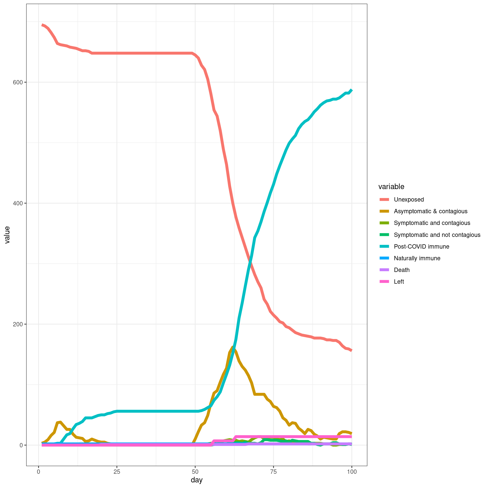
In this simulation, a travel ban is implemented from Day 7 and removed early (In this case from day 49). Each traveler will have only three connections with local agents
numDays = 100
enable_outside_travel_restriction_day <- 7
second_wave_day <- as.integer((49/100)*numDays)
#as.integer((numAgents_initial)*(1/100))
disthistory <- travel_ban_lift(enable_outside_travel_restriction_day,second_wave_day,
connection_number = 3,will_affect_traveler = 1,numDays = numDays )
## [1] "TOTAL"
## [1] 791
## [1] "Total Local"
## [1] 700
## [1] "Local Death"
## [1] 2
## [1] "-----"
## [1] "Total Traveler"
## [1] 91
## [1] "Traveler Death"
## [1] 0
## [1] "Local infected at somepoint"
## [1] 534
## [1] "Traveler infected at somepoint"
## [1] 83
## [1] "Total infected at somepoint"
## [1] 617 disthist.df <-as.data.frame(disthistory)
colnames(disthist.df) <- STATENAMES
disthist.df$day <- 1:nrow(disthistory)
histlong <- melt(disthist.df,id.vars="day")
ggplot(histlong,aes(x=day,y=value,fill=variable)) + geom_bar(stat="identity",position="stack") +
theme_bw()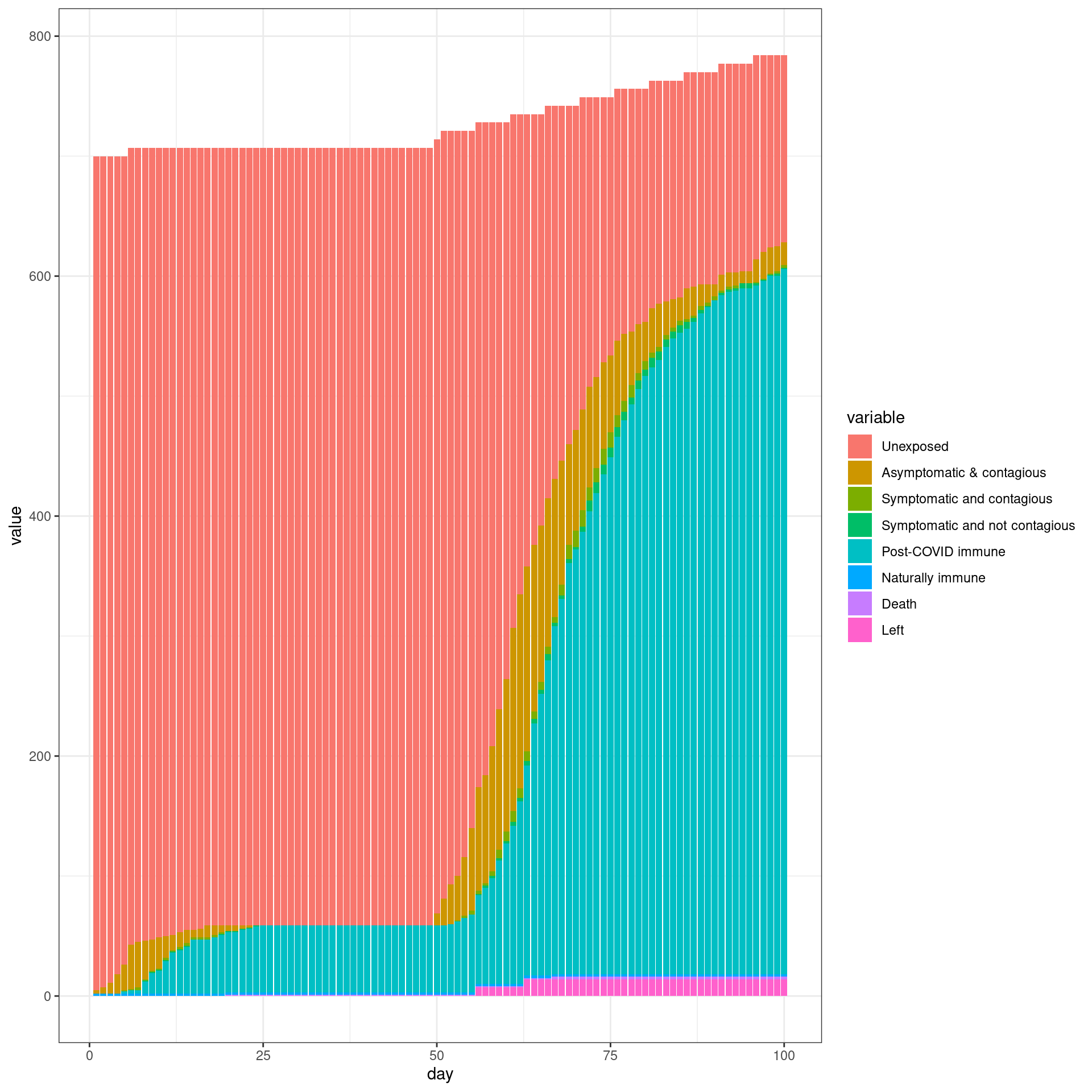
  ##make the SIR plot:
  sir <- data.frame(day=disthist.df$day,
                    susceptible = disthist.df$Unexposed,
                    infected = disthist.df[,2]+disthist.df[,3],
                    recovered = rowSums(disthist.df[,4:7]))

  ggplot(melt(sir,id.vars="day"),aes(x=day,group=variable,y=value,color=variable)) + geom_line(size=2) + theme_bw()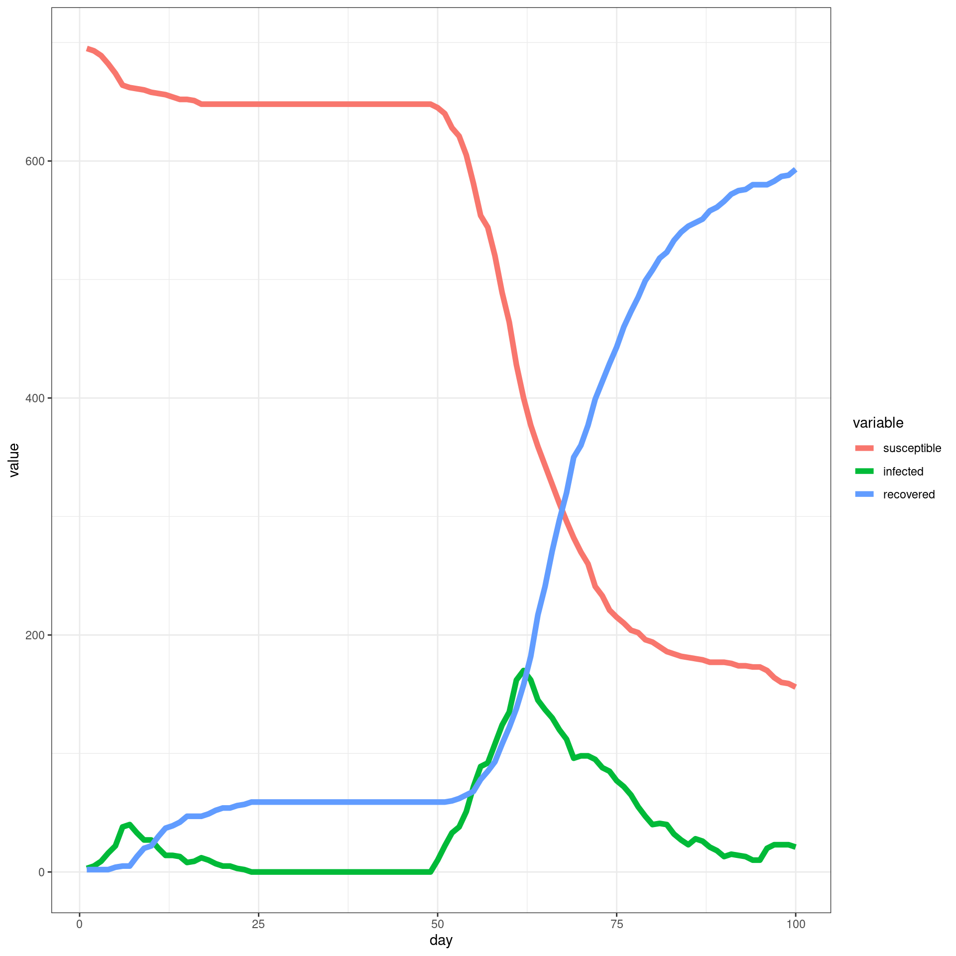
Travel ban/removed late
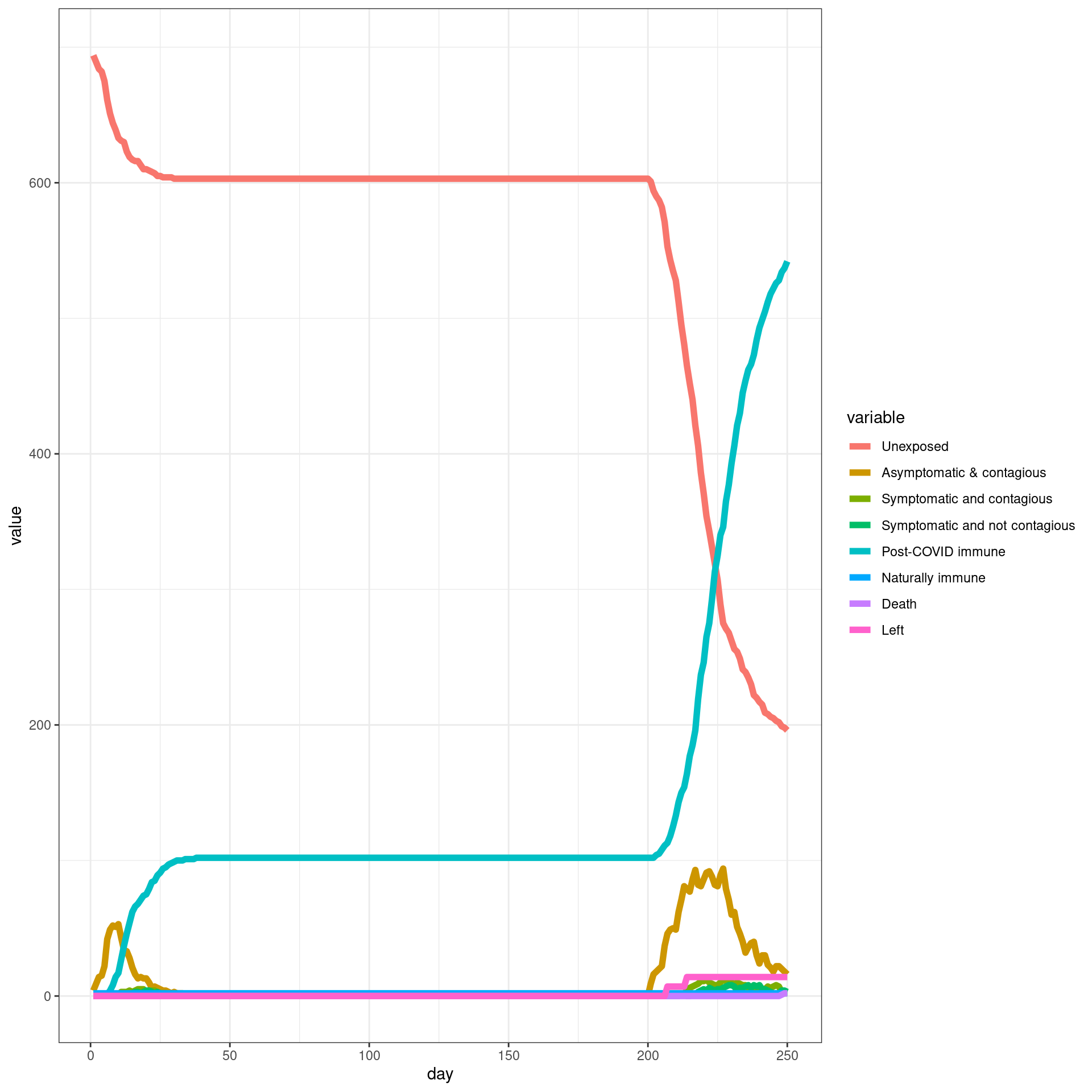
In this simulation, a ban is implemented from Day 7 and removed later. Each traveler will have only three connection with local agents
  numDays = 250
  enable_outside_travel_restriction_day <- 7
  second_wave_day <- as.integer((80/100)*numDays)

  #as.integer((numAgents_initial)*(1/100))
  disthistory <- travel_ban_lift(enable_outside_travel_restriction_day,second_wave_day,
                  connection_number = 3,will_affect_traveler = 1,numDays = numDays  )
## [1] "TOTAL"
## [1] 784
## [1] "Total Local"
## [1] 700
## [1] "Local Death"
## [1] 2
## [1] "-----"
## [1] "Total Traveler"
## [1] 84
## [1] "Traveler Death"
## [1] 0
## [1] "Local infected at somepoint"
## [1] 493
## [1] "Traveler infected at somepoint"
## [1] 77
## [1] "Total infected at somepoint"
## [1] 570 disthist.df <-as.data.frame(disthistory)
colnames(disthist.df) <- STATENAMES
disthist.df$day <- 1:nrow(disthistory)
histlong <- melt(disthist.df,id.vars="day")
ggplot(histlong,aes(x=day,y=value,fill=variable)) + geom_bar(stat="identity",position="stack") +
theme_bw() ##make the SIR plot:
sir <- data.frame(day=disthist.df$day,
susceptible = disthist.df$Unexposed,
infected = disthist.df[,2]+disthist.df[,3],
recovered = rowSums(disthist.df[,4:7]))
ggplot(melt(sir,id.vars="day"),aes(x=day,group=variable,y=value,color=variable)) + geom_line(size=2) + theme_bw()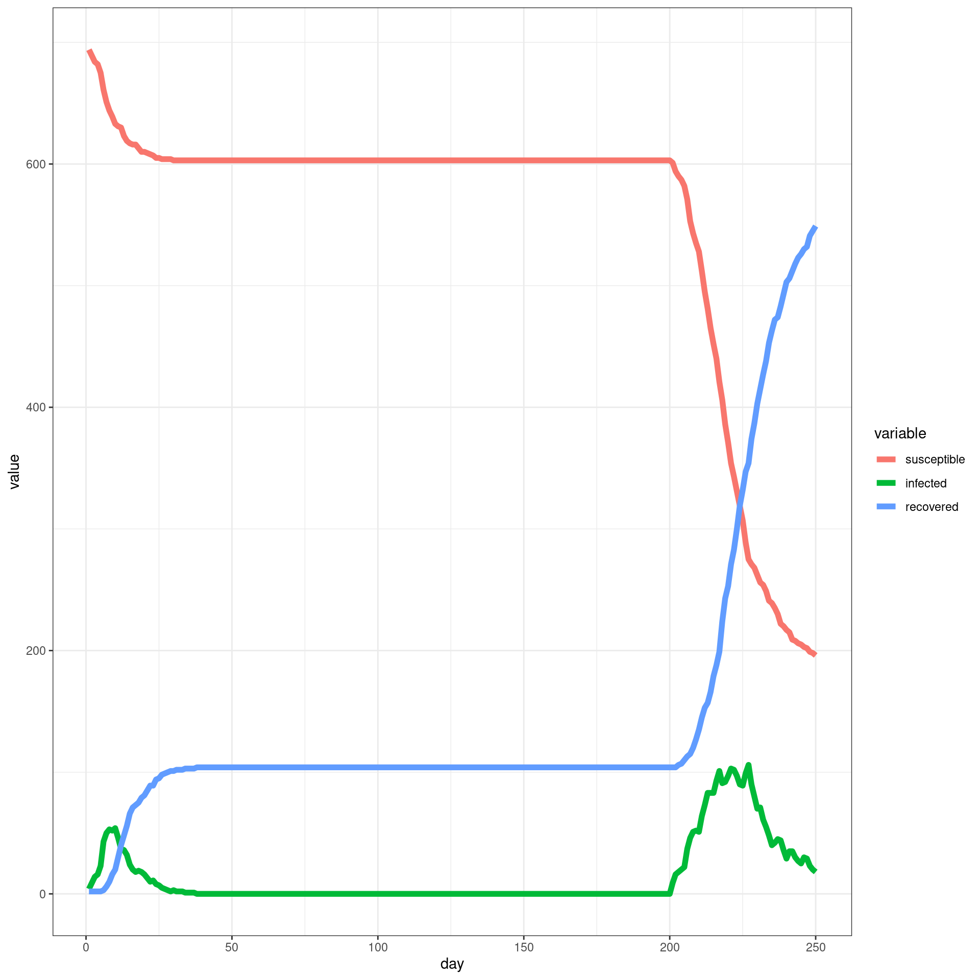
Social model
This is not quite right, because we’d really expect interactions to be clumpy–you interact with the same people every day, but this model is like the opinion dynamics model in that anyone can interact with anyone. Let’s make a network using preferential attachment to represent that social world. We can make a couple of them and add them together to represent how we each have different types of relationships and interactions–you may be the president of your drama club and so are a central member, but you are also in a pottery class where you don’t talk to very many people (although your teacher does).