Modeling psychological impacts on epidemic spread
Background
This markdown file goes through the basics of an agent-based model of epidemic spread. The model implements agents that progress through the disease in a series of stages, with the time required for each stage a random variable controlled by parameters of the model. The agent can have psychological states to allow exploring interactions, compliance, etc. Furthermore, we define a social network that governs the agent’s interaction patterns.
In this markdown file, we go through, step-by-step, the definition of the agent and the network, and give an initial simulation and look at the data.
Developing the agent
We will use a simplified task network model to represent the biological progression of the disease. First, let’s suppose that an agent has two states: its psychological state and its biological state. psychological state might be ‘practicing distancing’, ‘believes conspiracy theory’, ‘in quarantine’, and we can explore these later. Let’s just consider everyone is in a generic ‘informed’ state [1].
The biological state has a few specific cases:
- Unexposed
- Asymptomatic but infected/contagious
- Symptomatic and contagious
- Symptomatic and not contagious
- Post-COVID Immune
- Naturally immune (will not contract)
- Death
We could identify several others as well. Existing SIR models used for the COVID-19 epidemic often break #3 into 2-3 stages, ending in hospitalization and possibly death. With that stage, we could identify the hospital needs, but it will require estimating more parameters and having a more complex model. Initially, we can define the agent according to just a single biological value–the state it is in. We might assume that initially, most people are in bio-state 1, but some would be in state 6 already, which is essentially the same as state 5. we will also keep track of a psychological value as a placeholder.
To keep things simple, we will use some global variables to define the model, including the labels for these states.
##
## Attaching package: 'dplyr'
## The following objects are masked from 'package:stats':
##
## filter, lag## The following objects are masked from 'package:base':
##
## intersect, setdiff, setequal, union## Loading required package: statnet.common##
## Attaching package: 'statnet.common'## The following object is masked from 'package:base':
##
## order## Loading required package: network## network: Classes for Relational Data
## Version 1.16.0 created on 2019-11-30.
## copyright (c) 2005, Carter T. Butts, University of California-Irvine
## Mark S. Handcock, University of California -- Los Angeles
## David R. Hunter, Penn State University
## Martina Morris, University of Washington
## Skye Bender-deMoll, University of Washington
## For citation information, type citation("network").
## Type help("network-package") to get started.## sna: Tools for Social Network Analysis
## Version 2.5 created on 2019-12-09.
## copyright (c) 2005, Carter T. Butts, University of California-Irvine
## For citation information, type citation("sna").
## Type help(package="sna") to get started.##
## Attaching package: 'igraph'## The following objects are masked from 'package:sna':
##
## betweenness, bonpow, closeness, components, degree, dyad.census,
## evcent, hierarchy, is.connected, neighborhood, triad.census## The following objects are masked from 'package:network':
##
## %c%, %s%, add.edges, add.vertices, delete.edges, delete.vertices,
## get.edge.attribute, get.edges, get.vertex.attribute, is.bipartite,
## is.directed, list.edge.attributes, list.vertex.attributes,
## set.edge.attribute, set.vertex.attribute## The following objects are masked from 'package:dplyr':
##
## as_data_frame, groups, union## The following objects are masked from 'package:stats':
##
## decompose, spectrum## The following object is masked from 'package:base':
##
## unionSTATES <<- 7
STATENAMES <<- c("Unexposed",
"Asymptomatic & contagious",
"Symptomatic and contagious",
"Symptomatic and not contagious",
"Post-COVID immune",
"Naturally immune",
"Death")
STATELABELS <<- c("Unexposed","Asymptomatic\n & contagious",
"Symptomatic \n& contagious",
"Symptomatic \n& not contagious",
"Post-COVID immune",
"Naturally immune",
"Death")
makeAgent <- function(psych,bio)
{
return (list(psychstate=psych,biostate=bio))
}
print(makeAgent(1,2))## $psychstate
## [1] 1
##
## $biostate
## [1] 2We might augment the model to capture things like demographics (health, age). So lets add some more information. This information could involve things like geographical information, school membership, other risk factors, personality, belief in conspiracy theories, etc.
We will just define these as a named list.
makeAgent <- function(psych,bio,age=30)
{

  return (list(psychstate=psych,biostate=bio,age=age))
}
print(makeAgent(1,2))
## $psychstate
## [1] 1
##
## $biostate
## [1] 2
##
## $age
## [1] 30Timecourse of Biological model
Once infected, we will assume that the trajectory of the disease is essentially fixed and progresses, eventually leading to recovered or (in a small number) death. We need a way to transition the biological state automatically in a reasonable way, much like a task network model that keeps track of time of sub-events. This should consider ONLY the natural progression of the disease. We will model timecourse on a timecourse of 1-day units.
An easy way to do this is with ballistic events. That is, we can keep track of the next transition point for any state, if it is programmed at the beginning of the state. This let’s you use distributions other than an exponential/geometric distribution, because you can determine the stage duration at the beginning of the stage.
This creates a slightly more complex model and shows what it looks like:
makeAgent <- function(psychstate,biostate,age=30)
{

  return (list(psychstate=psychstate,
               biostate=biostate,
               age=age,
               nextbiostate=NA,
               biostatecountdown=NA))
}
print(makeAgent(1,2))
## $psychstate
## [1] 1
##
## $biostate
## [1] 2
##
## $age
## [1] 30
##
## $nextbiostate
## [1] NA
##
## $biostatecountdown
## [1] NATesting progression of biological model
We can prototype the information we need to progress through biological states. Here, when we set a state (infected), we also set the next state and when the next state will occur as a countdown timer. Alterately, we could identify the timepoint at which the change needs to be handled. This might be smarter if we had a larger more complex system, because we could keep track of only the next transitions more efficiently across a large number of agents and transition types. But here, we will just let each agent know when it should transation to the next stage.
set.seed(100)
agent <- makeAgent(psychstate=1, biostate=2)

##infect the agent
agent$biostate <- 1   ##infected but asymptomatic
agent$nextbiostate <- 2  ##infected and symptomitac/contageous
agent$biostatecountdown <- ceiling(abs(rnorm(1,mean=8,sd=1)))
print(agent)
## $psychstate
## [1] 1
##
## $biostate
## [1] 1
##
## $age
## [1] 30
##
## $nextbiostate
## [1] 2
##
## $biostatecountdown
## [1] 8Notice how this agent knows it is in biostate 1, and it will move to bio state 2 in 8 days.
##Updating the agent each day
Right now, although the agent is in state 1, it ‘knows’ it will transition to state 2 in, e.g., 8 days. We just need a function to update the agent’s state every day, change the countdown, and transition the agent to its next state if needed. If there is no next state (cured or dead), we will set the state to NA and no longer update.
updateAgent<- function(agent)
{
   agent$biostatecountdown <- agent$biostatecountdown -1
  if(agent$biostatecountdown <=0)
  {
    agent$biostate <- agent$nextbiostate
    agent$biostatecountdown <- NA
  }
   return(agent)
}
Now, we can run a loop, and on each day update the agent with the updateAgent function. Because R is functional, we need to return and replace the agent, which will ultimately make the model slower, and we might consider another approach eventually to scale the simulation up.
agent$biostate <- 1  ##Unexposed
agent$nextbiostate <- 2  ##asymptomatic but infected
agent$biostatecountdown <- ceiling(abs(rnorm(1,mean=8,sd=1)))
print(agent)
## $psychstate
## [1] 1
##
## $biostate
## [1] 1
##
## $age
## [1] 30
##
## $nextbiostate
## [1] 2
##
## $biostatecountdown
## [1] 9continue <- TRUE
while(continue)
{
print(paste(agent$biostate,agent$biostatecountdown))
agent <- updateAgent(agent)
continue <-!is.na(agent$biostatecountdown)
}## [1] "1 9"
## [1] "1 8"
## [1] "1 7"
## [1] "1 6"
## [1] "1 5"
## [1] "1 4"
## [1] "1 3"
## [1] "1 2"
## [1] "1 1"Create transition matrix.
Now that we have a way of transitioning between states, we need to implement the entire set of possible transitions and the timing of each stage. To keep it simple, we will make all timing distributions uniform with a min and max parameter for time in each state. We can program several possible pathways through the stages, with a couple branch points (death vs recovery; the possibility of recovering after acquiring with no symptoms). The progression of the disease is completely specified by this data, and a generic update function will then automatically progress the agent each day.
Along with the main data, we will create functions that set and update the agent state.
# * 1. Unexposed
# * 2. Asymptomatic but infected/contagious
# * 3. Symptomatic and contagious
# * 4. Symptomatic and not contagious
# * 5. Post-COVID Immune
# * 6. Naturally immune (will not contract)
# * 7. Death


bioTransition <- matrix(0,STATES,STATES)
bioMin <- matrix(1,STATES)      #state time minimum
bioMax <- matrix(1,STATES)      #state time maximum


bioMin[2] <- 3            #infected but asymptomatic for 3 to 10 days
bioMax[2] <- 10
bioTransition[2,3] <- .5  #transition to infected with symptoms
bioTransition[2,5] <- .5  #transition to no longer contagious/cured


bioMin[3] <-    3             #symptoms + contagion
bioMax[3] <- 8                #symptoms + contagion max
bioTransition[3,4] <-  .95    #transitioon to no longer contagious
bioTransition[3,7] <-  .05    #transitioon to death state


bioMin[4] <- 1          #symptoms bot no longer contagiious
bioMax[4] <- 7
bioTransition[4,5] <- 1  #Transition to 'immune' cured state.


setAgentState<- function(agent, biostate)
{
  agent$biostate <- biostate
  if(sum(bioTransition[biostate,])>0) # this state transitions to something else.
  {
    ##which state do we go to?
     agent$biostatecountdown <- sample(x=seq(bioMin[biostate],bioMax[biostate]),1) #how long will we state in this state?
     agent$nextbiostate <- sample(1:STATES, prob=bioTransition[agent$biostate,],size=1)

  } else{
   agent$biostatecountdown <- NA
   agent$nextbiostate <- NA   ##just so we can tell if the agent is finished.
  }
  return(agent)
}

transitionAgent<- function(agent)
{
   return(setAgentState(agent,agent$nextbiostate))
}

updateAgent<- function(agent)
{
  if(!is.na(agent$biostatecountdown))
  {
   agent$biostatecountdown <- agent$biostatecountdown -1
    if(agent$biostatecountdown <=0)  ##new state
    {
       agent <- transitionAgent(agent)

    }
  }
   return(agent)
}
Because the biological state system is a network, we can visualize with the gplot function in the sna library:
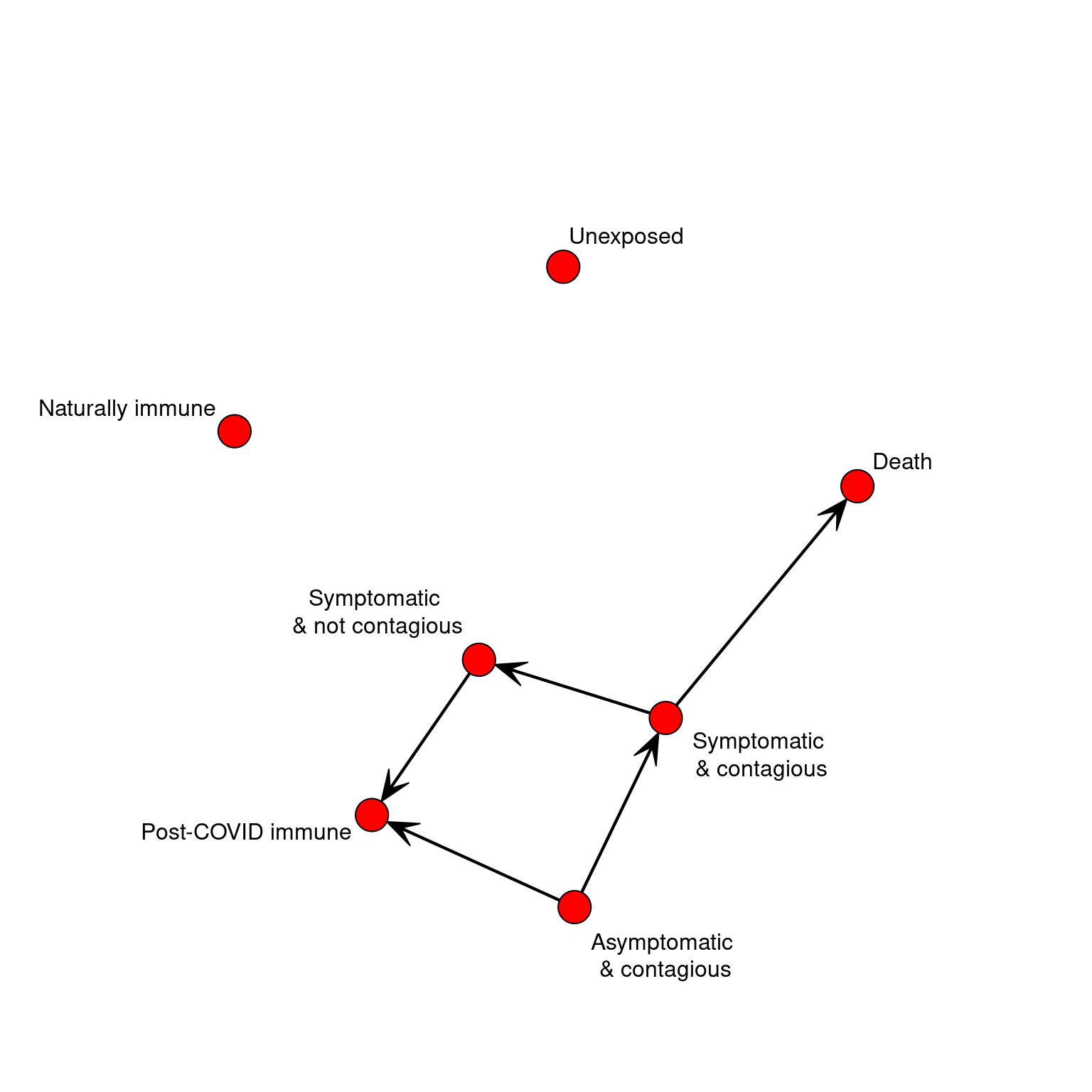
If we start an agent in an unexposed state, nothing happens. Agent’s do not just naturally develop the disease. We can just update the agent until there is no next-state programmed.
agent <- makeAgent(psychstate=1,biostate=1)

continue <- TRUE
while(continue)
{
  print(paste(agent$biostate,STATENAMES[agent$biostate],agent$biostatecountdown))
  agent <- updateAgent(agent)
  continue <-!is.na(agent$nextbiostate)
}
## [1] "1 Unexposed NA"If we infect a patient, the entire disease progression will occur. Run several times to see the different alternative possibilities.
agent <- makeAgent(psychstate=1,biostate=1)
agent <- setAgentState(agent,2)##infect!
continue <- TRUE

time <- 1
while(continue)
{

  print(paste(time,agent$biostate,STATENAMES[agent$biostate],agent$biostatecountdown))
  agent <- updateAgent(agent)
  continue <-!is.na(agent$nextbiostate)
  time <- time + 1
}
## [1] "1 2 Asymptomatic & contagious 6"
## [1] "2 2 Asymptomatic & contagious 5"
## [1] "3 2 Asymptomatic & contagious 4"
## [1] "4 2 Asymptomatic & contagious 3"
## [1] "5 2 Asymptomatic & contagious 2"
## [1] "6 2 Asymptomatic & contagious 1"
## [1] "7 3 Symptomatic and contagious 7"
## [1] "8 3 Symptomatic and contagious 6"
## [1] "9 3 Symptomatic and contagious 5"
## [1] "10 3 Symptomatic and contagious 4"
## [1] "11 3 Symptomatic and contagious 3"
## [1] "12 3 Symptomatic and contagious 2"
## [1] "13 3 Symptomatic and contagious 1"
## [1] "14 4 Symptomatic and not contagious 2"
## [1] "15 4 Symptomatic and not contagious 1"## [1] "5 Post-COVID immune NA"Basic social model
Now that we have the biological disease model whose stages we can control (and it has branches too.) We can infect an agent or deliberately change its state. Now, let’s put this is a population. We will assume a flat organization where everyone has an equal chance of interacting with everyone else. Here, the parameters are:
- ‘numAgents’: how many agents are in the simulation. This simulation cannot easily handle more than around 1000. Even with a fast computer, you might simulate 5000 and it will take 20 minutes or more. To simulate a larger realistic population, we would need to re-implement some of the data and algorithms.
- ‘naturalImmunity’: This controls the proportion who will never get the disease at the beginning of the simulation.
- ‘numInteractions’: how many interactions do each agent make every day?
- ‘numDays’: how many days to simulate?
- ‘contagionProb’: how likely is the disease to spread when an infected agent interacts with a susceptible agent?
We will also keep track of the the distribution each day in the matrix disthistory. We will start the simulation by infecting a small number of agents (here, 3) using setAgentState() function.
set.seed(100)
numAgents <- 500
naturalImmunity <- .01  #1 % naturally immune
numInteractions <-  10 ##how many interactions per day per agent on average?
numDays <- 50
contagionProb <- .1    ##normal contagion probability


disthistory <- matrix(NA,ncol=STATES,nrow=numDays)

pool <- list()
for(i in 1:numAgents)
{
  pool[[i]] <- makeAgent(psychstate=1,
                         biostate=sample(c(1,6),
                          p=c(1-naturalImmunity, naturalImmunity),1))
}

##infect patients 0
numInfected <- 3
for(i in sample(numAgents,numInfected))
{
   pool[[i]] <- setAgentState(pool[[i]],2) ##infect this person
}

for(day in 1:numDays)
{
##who are you going to talk to today.
    sneezeOn <- cbind(rep(1:numAgents,each=numInteractions),
                      sample(numAgents,replace=T,size=numAgents*numInteractions))


  for(i in 1:nrow(sneezeOn))
  {
    agent1 <- pool[[ sneezeOn[i,1] ]]
    agent2 <- pool[[ sneezeOn[i,2] ]]

    if((agent1$biostate==2 || agent1$biostate==3 ) & agent2$biostate==1 & runif(1)<contagionProb)
    {
      pool[[ sneezeOn[i,2] ]] <- setAgentState(agent2,2)##infect!
    }

  }
    ##increment each agent 1-day.
    for(i in 1:numAgents)
    {
      pool[[i]] <- updateAgent(pool[[i]])
    }

    distrib <- table(factor(sapply(pool,FUN=function(x){x$biostate}),levels=1:7))
    disthistory[day,] <- distrib

}

#barplot(t(disthistory),col=1:7)
disthist.df <-as.data.frame(disthistory)
colnames(disthist.df) <- STATENAMES
disthist.df$day <- 1:nrow(disthistory)


show <- disthist.df[c(1,5*(1:(day/5))),c(8,1:7)]
print(kable(show))
##
##
## day Unexposed Asymptomatic & contagious Symptomatic and contagious Symptomatic and not contagious Post-COVID immune Naturally immune Death
## --- ---- ---------- -------------------------- --------------------------- ------------------------------- ------------------ ----------------- ------
## 1 1 480 11 0 0 0 9 0
## 5 5 255 223 8 0 5 9 0
## 10 10 3 264 106 11 107 9 0
## 15 15 0 31 131 76 250 9 3
## 20 20 0 0 33 86 365 9 7
## 25 25 0 0 1 21 459 9 10
## 30 30 0 0 0 0 481 9 10
## 35 35 0 0 0 0 481 9 10
## 40 40 0 0 0 0 481 9 10
## 45 45 0 0 0 0 481 9 10
## 50 50 0 0 0 0 481 9 10histlong <- melt(disthist.df,id.vars="day")
ggplot(histlong,aes(x=day,y=value,fill=variable)) + geom_bar(stat="identity",position="stack") +
theme_bw()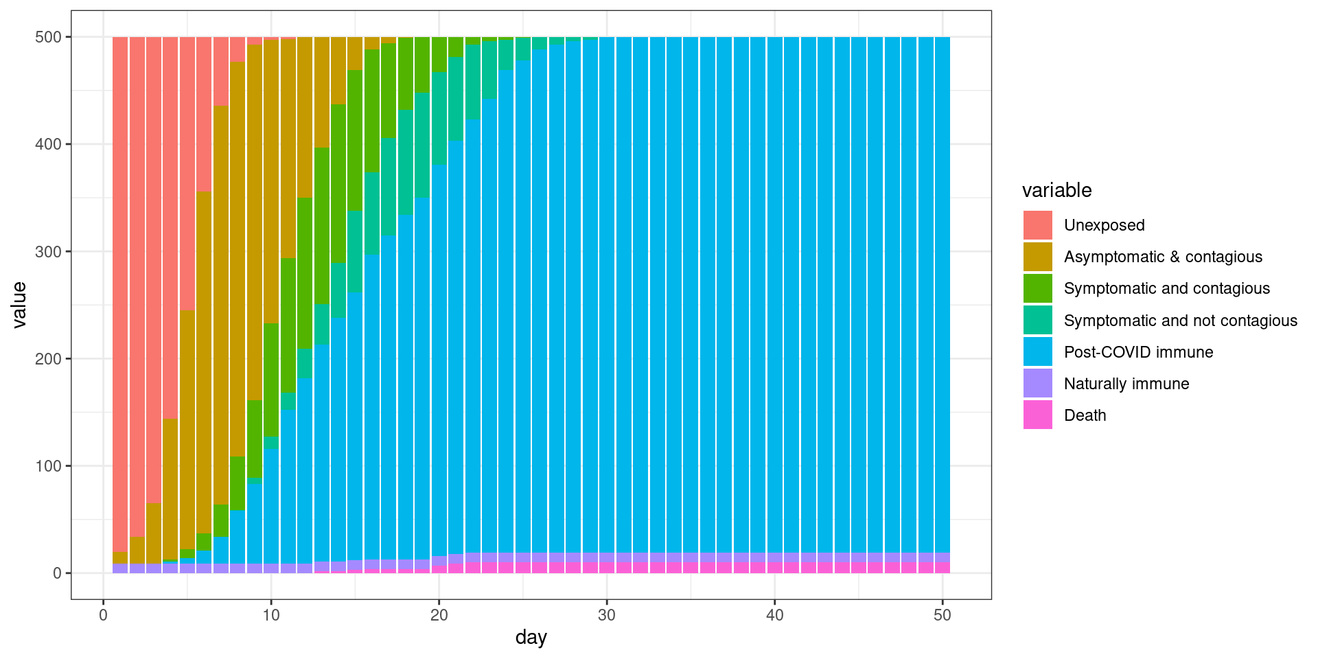
##make the SIR plot:
sir <- data.frame(day=disthist.df$day,
susceptible = disthist.df$Unexposed,
infected = disthist.df[,2]+disthist.df[,3],
recovered = rowSums(disthist.df[,4:7]))
plot0 <- ggplot(melt(sir,id.vars="day"),aes(x=day,group=variable,y=value,color=variable)) + geom_line() + theme_bw() + ggtitle(label="Initial model with complete contact between agents")
print(plot0)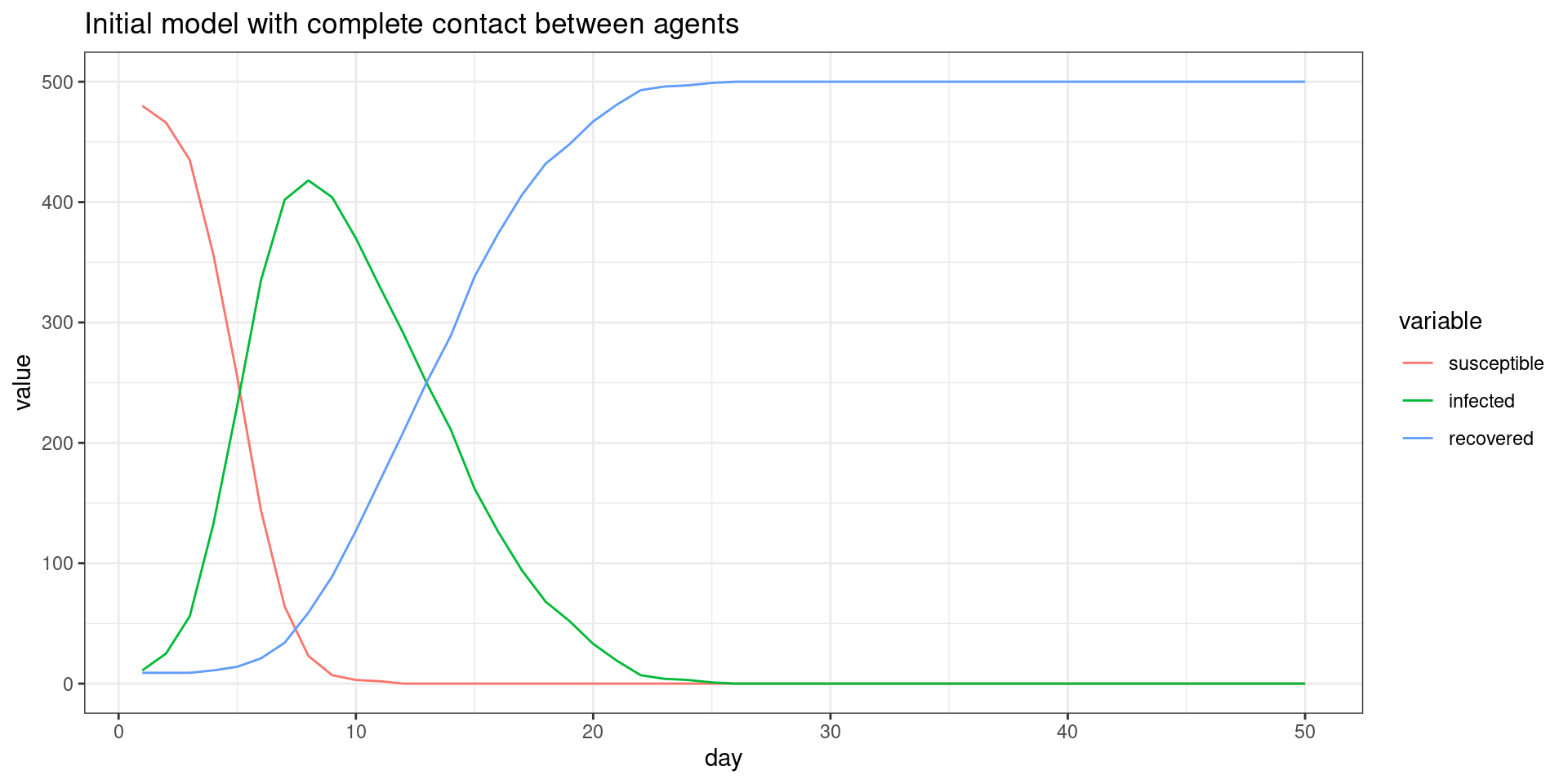
In this simulation, we can see the ‘infected’ proportion quickly rises, and within about 25 days the entire population has had the disease. We can also look at the daily change, which are the numbers that are often reported, at least to a first approximation. This is “the curve” that we would like to flatten.
cases <- sir$infected+sir$recovered
cases.daily <- cases[-1] - cases[-length(cases)]
plot(cases.daily,type="h",xlab="Day",ylab="Daily new cases")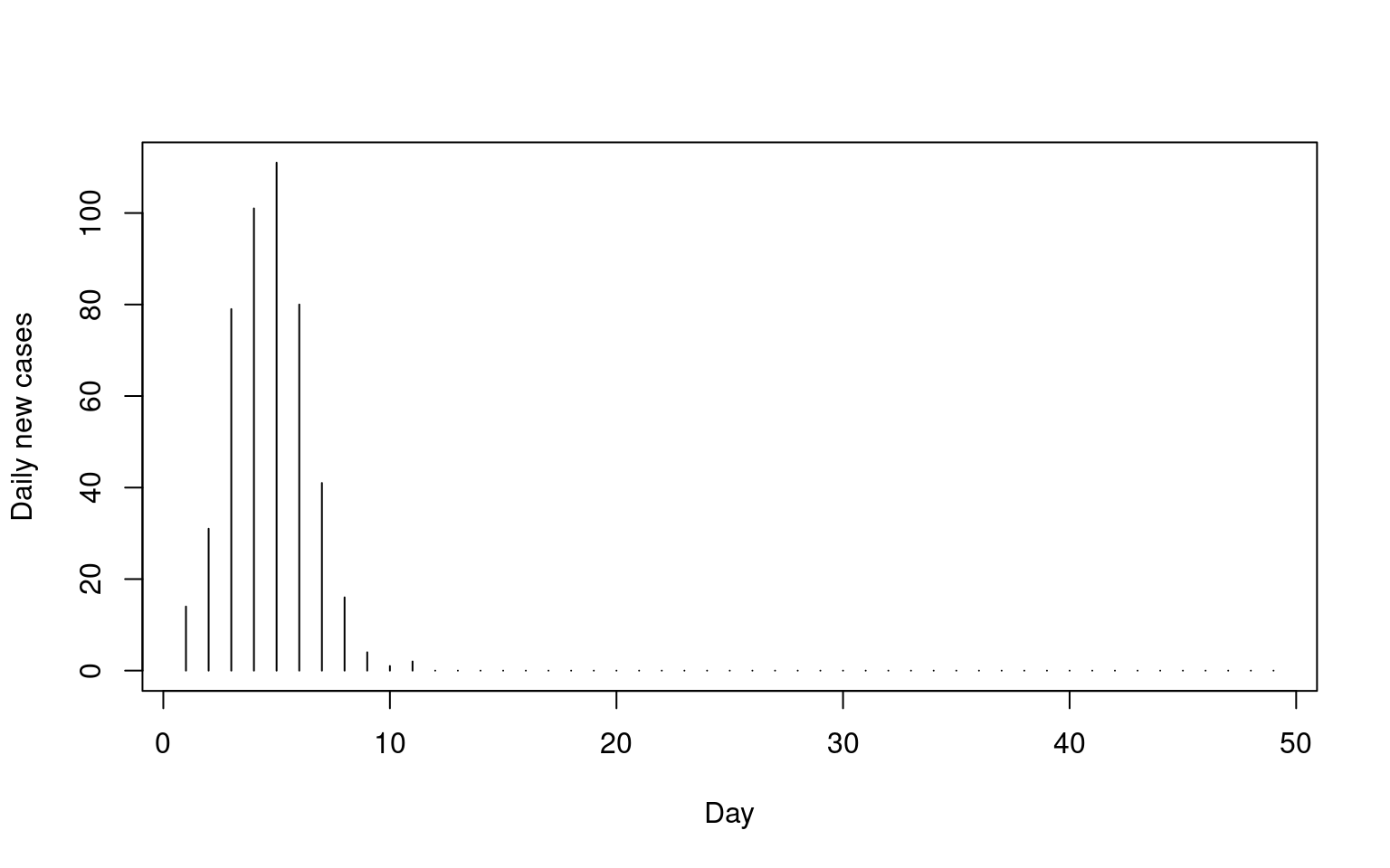
This captures the steep rise initially, followed by an asymptote. It also captures the phenomena that not all people get infected–here we end at around 75%.
Incorporating a social network into the model
This is not quite right, because we’d really expect interactions to be clumpy–you interact with the same people every day, but this model is like the opinion dynamics model in that anyone can interact with anyone. Let’s make a network using preferential attachment to represent that social world. We can make a couple of them and add them together to represent how we each have different types of relationships and interactions–you may be the president of your drama club and so are a central member, but you are also in a pottery class where you don’t talk to very many people (although your teacher does).
The following function will create a network from numsets independent smallworld networks. In addition, it will create direct connections between any agents steps links apart, to make the network more clumpy. the network shown is a single network with 2 steps. For some reason, the gplot function in sna is pretty slow, so we will re-write it to display our networks much more quickly.
makeNetwork<- function(numAgents,numsets=3,steps=1,power=1)
{
ord <- sample(numAgents)
tmp<-as_adjacency_matrix(sample_pa(numAgents,power=power),sparse=F)
tmp <- tmp + t(tmp)
tmp <- tmp[ord,ord]
if(numsets>1)
{
for(i in 2:numsets)
{
ord <- sample(numAgents)
sn2 <-as_adjacency_matrix(sample_pa(numAgents,power=power),sparse=F)[ord,ord]
tmp <- tmp + sn2 + t(sn2)
}
}
if(steps>1)
{
for(i in 2:steps)
{
tmp <- tmp + tmp %*% tmp ## iterate to neighbors
}
}
(tmp>0)+0
}
mygplot <- function(coord, network,states,main="")
{
if(is.null(coord))
{
coord <- gplot.layout.fruchtermanreingold(network,layout.par=list(niter=500))
}
newmin <- mean(coord[,2]) - (-min(coord[,2]) + mean(coord[,2])) * 1.4
palette=c("white","yellow","red","green","darkgreen","blue","black")
plot(coord,col="black",bty="n",pch=16,cex=2.7,xaxt="n",yaxt="n",main=main,xlab="",ylab="",axes=F,
ylim=c(newmin,max(coord[,2])),type="n")
for(i in 1:nrow(network))
segments(coord[i,1],
coord[i,2],
coord[network[i,]==1,1],
coord[network[i,]==1,2],col="grey40")
points(coord,pch=16,cex=2.3,col= palette[states])
points(coord,pch=1,cex=2.3,col="black")
legend(mean(coord[,1]),min(coord[,2]),bty='n',y.intersp=.7,cex=.8,
STATENAMES, pch=16,col=palette)
return (coord)
}
set.seed(100)
socialnetwork <- makeNetwork(1000,numsets=1,power=.59,steps=2)
cc <- mygplot(coord=NULL,socialnetwork,rep(1,nrow(socialnetwork)),main="Initial state")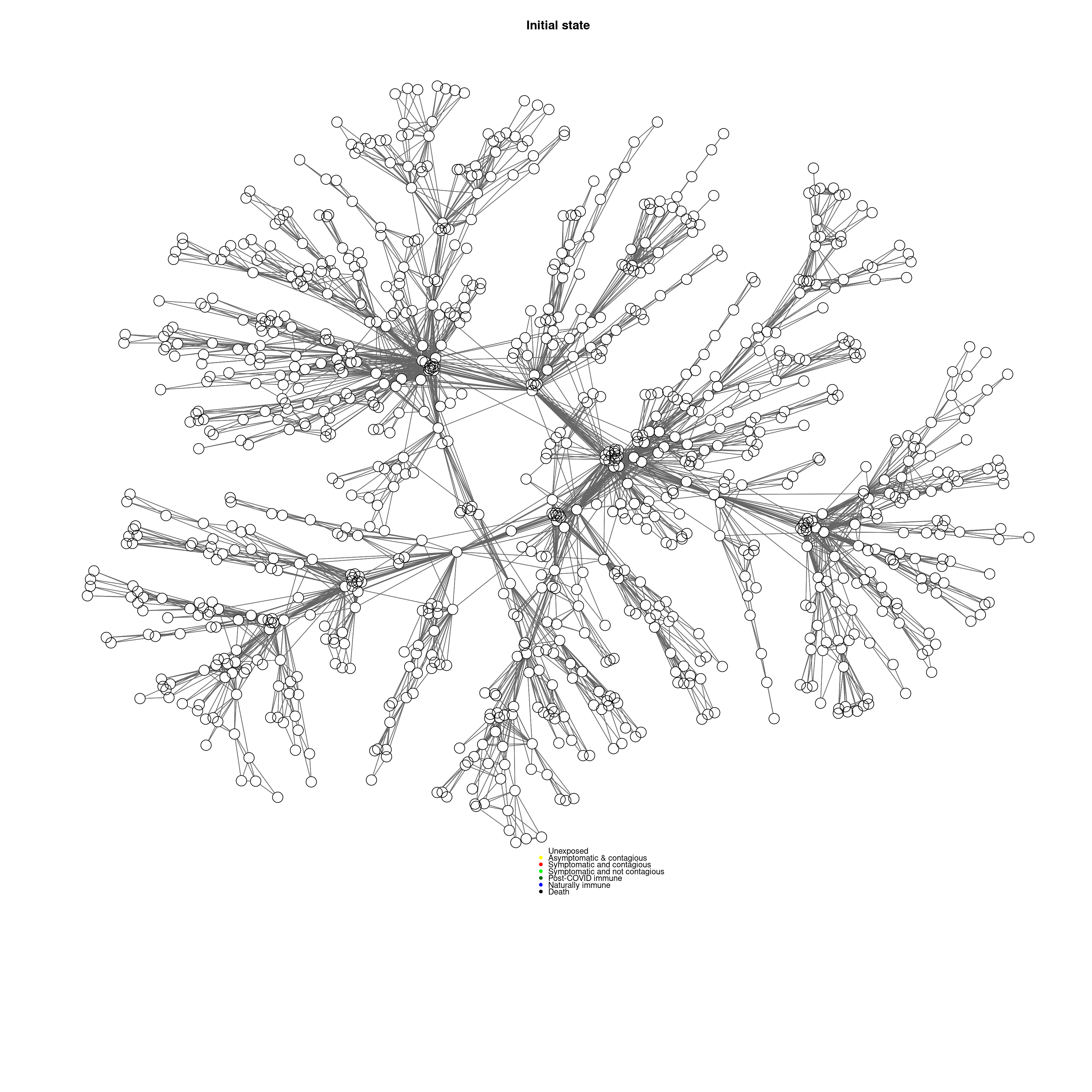
Now, let’s just say that we sample interactions MOSTLY from this network. For example 90% of interactions come from the network, and 10% are random, which would represent mostly-contact with your direct family, while 50-50 would involve much more community contact. This lets us automatically combine a network probabilistically with a random one.
Simulating with a social network.
Now, we can run the same simulation, using the social network with more limited connections.
set.seed(100)
numAgents <- 500
naturalImmunity <- .01 #1 % naturally immune
numInteractions <- 10 ##how many interactions per day per agent on average?
numDays <- 50
contagionProb <- .1 ##normal contagion probability
sampleFromNetwork <- .98
plotNetwork <-T
socialnetwork <-makeNetwork(numAgents,numsets=1,power=.5,steps=2)
if(plotNetwork)
{
cc <-mygplot(coord=NULL,socialnetwork,rep(1,nrow(socialnetwork)),main="Initial state")
} disthistory <- matrix(NA,ncol=STATES,nrow=numDays)
pool <- list()
for(i in 1:numAgents)
{
pool[[i]] <- makeAgent(psychstate=1,
biostate=sample(c(1,6),
p=c(1-naturalImmunity, naturalImmunity),1))
}
##infect patient 0
numInfected <- 3
for(i in sample(numAgents,numInfected))
{
pool[[i]] <- setAgentState(pool[[i]],2) ##infect this person
}
set.seed(100) #reset simulation seed so it is the same as previous.
for(day in 1:numDays)
{
##who are you going to talk to today.
sneezers <- rep(1:numAgents,each=numInteractions)
sneezedons <- rep(NA,length(sneezers))
for(i in 1:length(sneezers))
{
if(runif(1)<(1-sampleFromNetwork))
{
sneezedons[i] <- sample(numAgents,1)
}else{
sneezedons[i] <- sample(1:numAgents,prob=socialnetwork[sneezers[i],],1)
}
}
for(i in 1:length(sneezers))
{
agent1 <- pool[[ sneezers[i] ]]
agent2 <- pool[[ sneezedons[i] ]]
##this constitutes the rules of infection.
if((agent1$biostate==2 || agent1$biostate==3 ) & agent2$biostate==1 & runif(1)<contagionProb)
{
pool[[ sneezedons[i] ]] <- setAgentState(agent2,2)##infect!
}
}
##increment each agent 1-day.
for(i in 1:numAgents)
{
pool[[i]] <- updateAgent(pool[[i]])
}
states <- sapply(pool,FUN=function(x){x$biostate})
distrib <- table(factor(states,levels=1:7))
disthistory[day,] <- distrib
if(plotNetwork)
{
mygplot(cc,socialnetwork,states,main=paste("Day",day))
}
}
With the same starting configuration, we can see that the infection rate is slower, and in fact a few people remain uninfected after 50 days. This code animates the model over time (this makes the simulation take longer), and we can see that it spreads on branches. People who escape infection on a branch cannot easily be reached, and ultimately may be spared.
disthist.df <-as.data.frame(disthistory)
colnames(disthist.df) <- STATENAMES
disthist.df$day <- 1:nrow(disthistory)
histlong <- melt(disthist.df,id.vars="day")

ggplot(histlong,aes(x=day,y=value,fill=variable)) + geom_bar(stat="identity",position="stack") +
  theme_bw()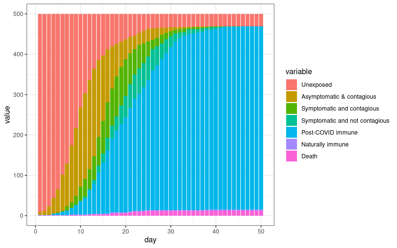
##make the SIR plot:
sir <- data.frame(day=disthist.df$day,
                  susceptible = disthist.df$Unexposed,
                  infected = disthist.df[,2]+disthist.df[,3],
                  recovered = rowSums(disthist.df[,4:7]))

plot1 <- ggplot(melt(sir,id.vars="day"),aes(x=day,group=variable,y=value,color=variable)) + geom_line() + theme_bw() + ggtitle(label="Social network model")
print(plot1)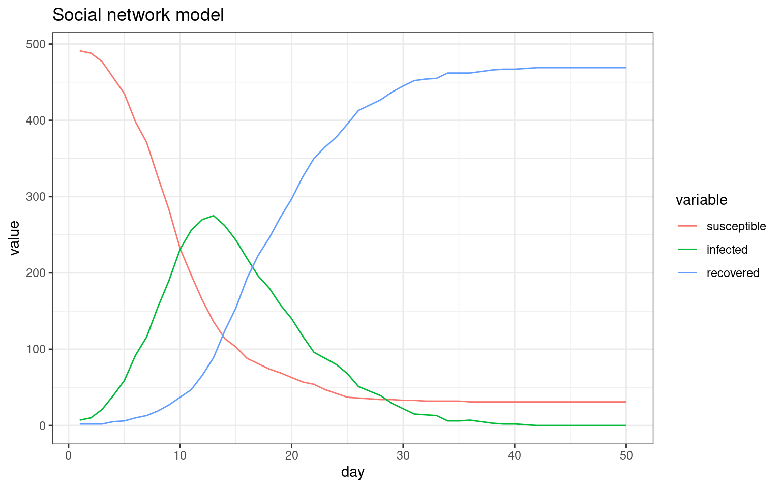

Changing behavior based on disease state
We can now start asking other questions. For example, what if the symptomatic people do not interact anymore? This just means re-writing the code where people get infected. This is probably realistic–when you get infected, you stay at home and stop interacting. It may be the case that those you interact with have a higher chance of getting the disease if you are sneezing and coughing, but we will keep the contagionProb the same.
set.seed(100)
numAgents <- 500
naturalImmunity <- .01  #1 % naturally immune
numInteractions <-  10 ##how many interactions per day per agent on average?
numDays <- 50
contagionProb <- .1    ##normal contagion probability
sampleFromNetwork <- .98


plotNetwork <- FALSE

socialnetwork <-makeNetwork(numAgents,numsets=1,power=.5,steps=2)
if(plotNetwork)
{
  cc <-mygplot(coord=NULL,socialnetwork,rep(1,nrow(socialnetwork)),main="Initial state")

}

  disthistory <- matrix(NA,ncol=STATES,nrow=numDays)

pool <- list()
for(i in 1:numAgents)
{
   pool[[i]] <- makeAgent(psychstate=1,
                         biostate=sample(c(1,6),
                          p=c(1-naturalImmunity, naturalImmunity),1))
}

##infect patient 0
numInfected <- 3
for(i in sample(numAgents,numInfected))
{
   pool[[i]] <- setAgentState(pool[[i]],2) ##infect this person
}

for(day in 1:numDays)
{
##who are you going to talk to today.
    sneezers <- rep(1:numAgents,each=numInteractions)
    sneezedons <- rep(NA,length(sneezers))

    for(i in 1:length(sneezers))
      {
      if(runif(1)<(1-sampleFromNetwork) )
      {
        sneezedons[i] <- sample(numAgents,1)
      }else{
        sneezedons[i] <- sample(1:numAgents,prob=socialnetwork[sneezers[i],],1)
      }
     }

  for(i in 1:length(sneezers))
  {
    agent1 <- pool[[ sneezers[i] ]]
    agent2 <- pool[[ sneezedons[i] ]]


    ##this constitutes the rules of infection.
    if((agent1$biostate==2 ) & agent2$biostate==1 & runif(1)<contagionProb)
    {
         pool[[ sneezedons[i] ]] <- setAgentState(agent2,2)##infect!
    }

  }
    ##increment each agent 1-day.
    for(i in 1:numAgents)
    {
      pool[[i]] <- updateAgent(pool[[i]])
    }

    states <- sapply(pool,FUN=function(x){x$biostate})
    distrib <- table(factor(states,levels=1:7))
    disthistory[day,] <- distrib
   if(plotNetwork)
   {
       mygplot(cc,socialnetwork,states,main=paste("Day",day))

   }


}

#barplot(t(disthistory),col=1:7)
disthist.df <-as.data.frame(disthistory)
colnames(disthist.df) <- STATENAMES
disthist.df$day <- 1:nrow(disthistory)
histlong <- melt(disthist.df,id.vars="day")
ggplot(histlong,aes(x=day,y=value,fill=variable)) + geom_bar(stat="identity",position="stack") +
theme_bw()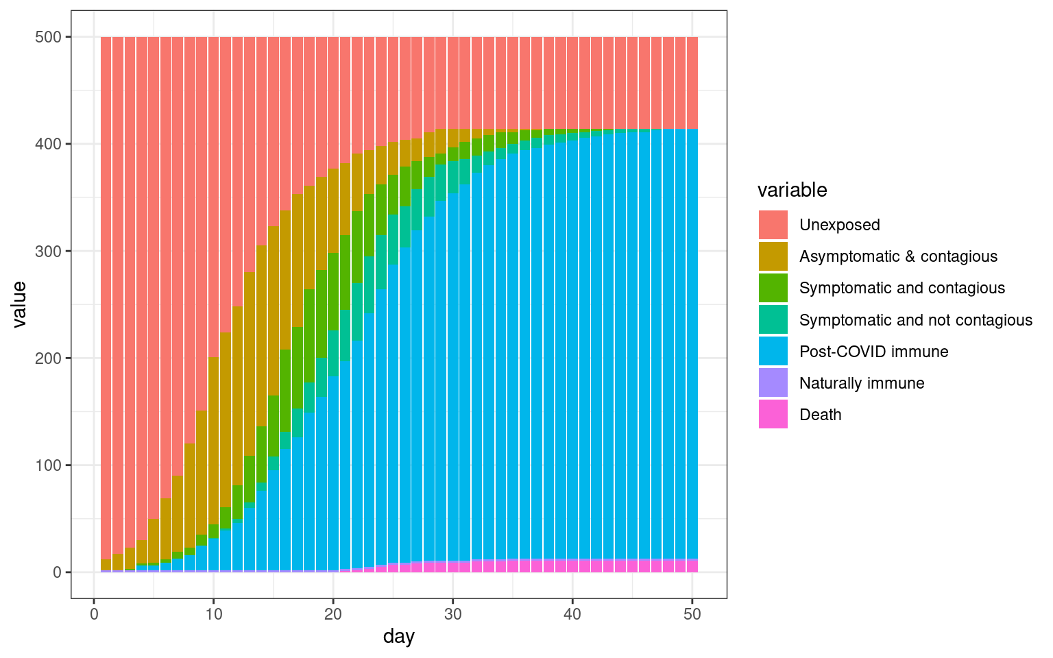
##make the SIR plot:
sir <- data.frame(day=disthist.df$day,
                  susceptible = disthist.df$Unexposed,
                  infected = disthist.df[,2]+disthist.df[,3],
                  recovered = rowSums(disthist.df[,4:7]))

plot2 <- ggplot(melt(sir,id.vars="day"),aes(x=day,group=variable,y=value,color=variable)) + geom_line() + theme_bw() + ggtitle(label="Social network model with limited contact once symptomatic")
print(plot2)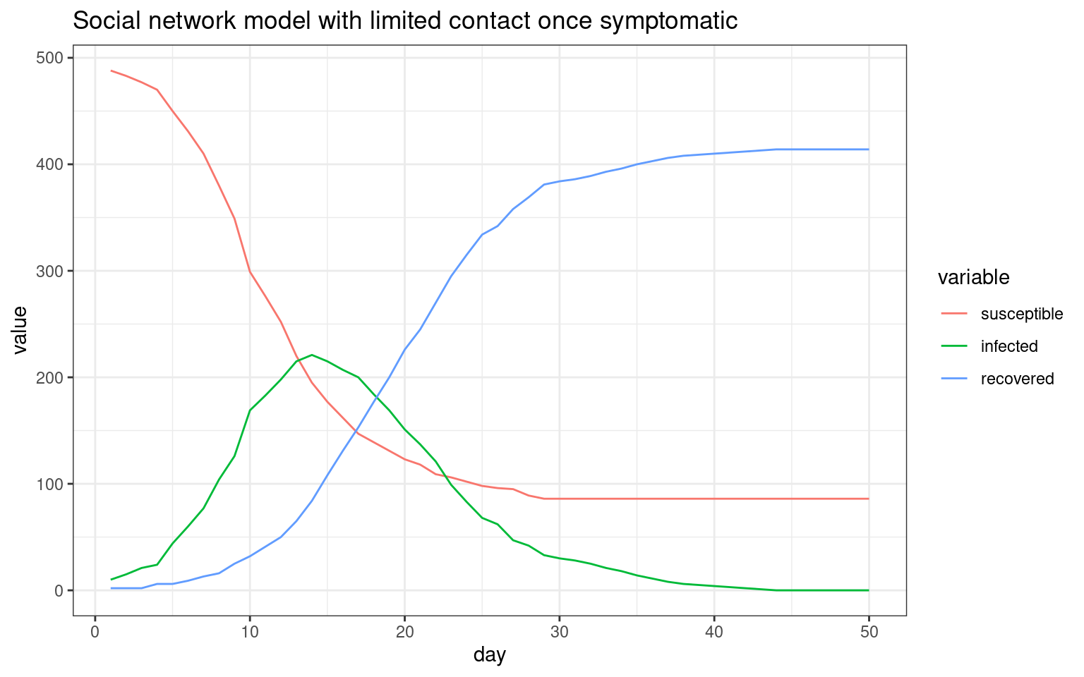
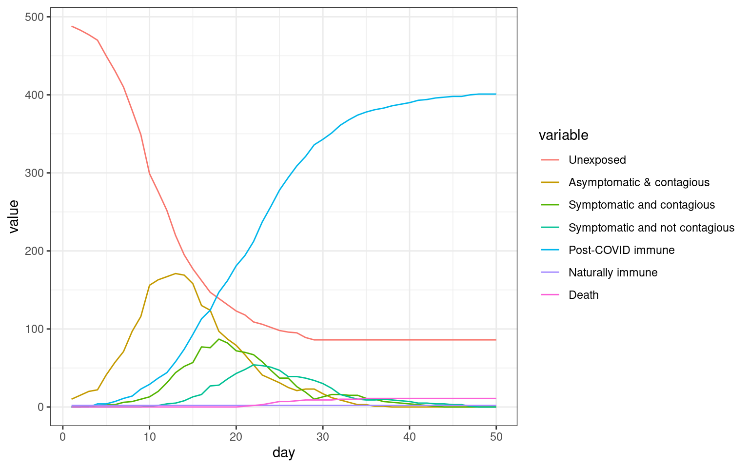 ## Comparing the three models This seems to be a decent starting point model for furher exploration. Here, the symptomatic people completely quarantine. That is, they decline all interaction and so do not spread the virus. All spreading is done by asymptomatics.
We can compare these three simulations because I saved the plot functions. Now we can see how each of these change the outcome of the model, showing assumptions about who is interacting with who, and during what stage, do indeed matter. These are difficult to implement without an agent-based model, and most of the current COVID-19 models do not consider these things.
##
## Attaching package: 'gridExtra'
## The following object is masked from 'package:dplyr':
##
## combine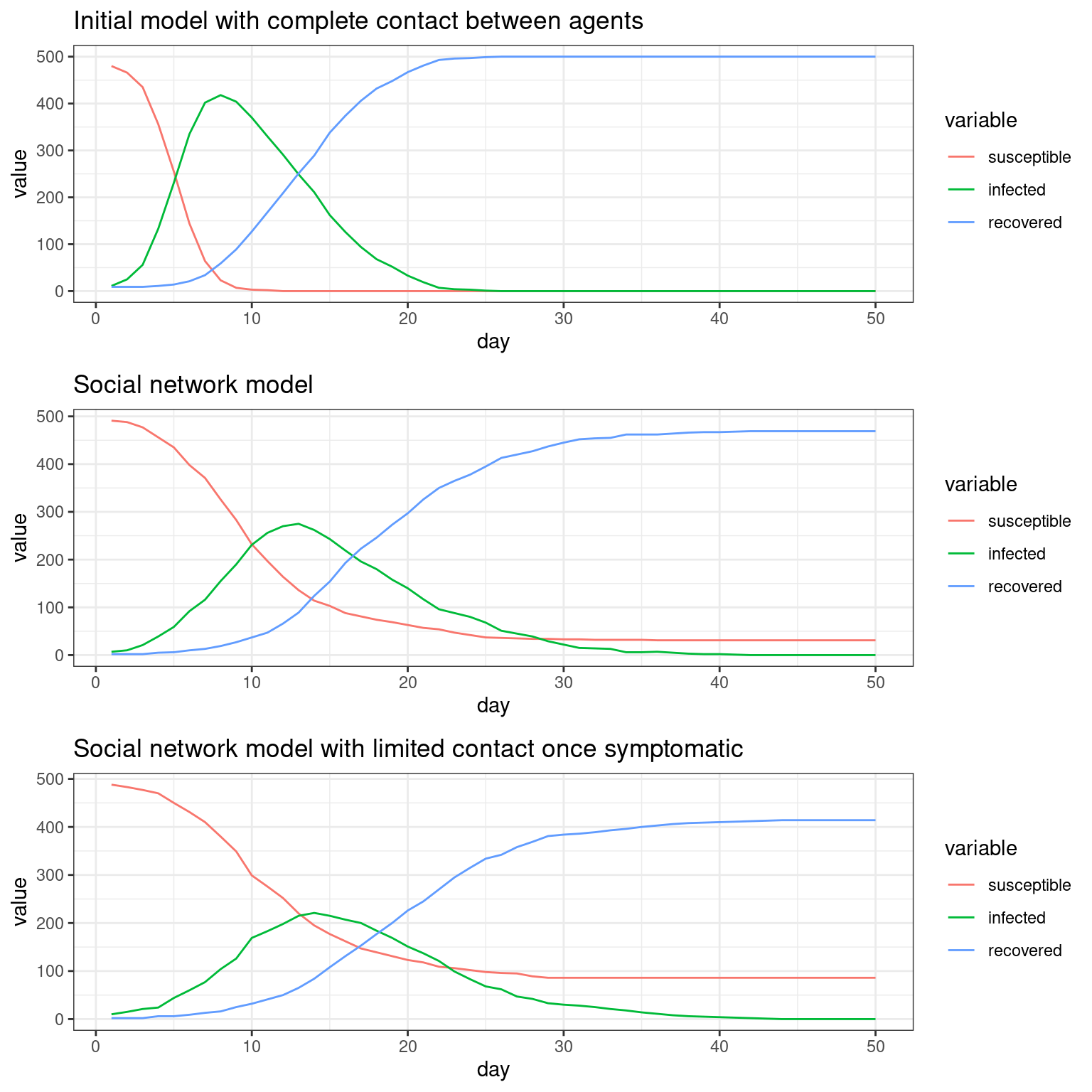
Modeling policy changes
We can try also change parameters or settings for some number of days; like a shelter-in-place order and lift, to explore how social or gov’t actions might influence behaviors. To do this, we will create a vector of parameters, to allow us to use a different parameter each day. To start, we will just change the number of interactions, to simulate a stay-at-home order and lift.
set.seed(100)
numAgents <- 500
naturalImmunity <- .01  #1 % naturally immune
numInteractions <-  10 ##how many interactions per day per agent on average?
numDays <- 50


socialnetwork <-makeNetwork(numAgents,numsets=1,power=.5,steps=2)

numInteractions <-  rep(10,numDays)  ##how many interactions per day per agent on average?
contagionProb <- rep(.1,numDays)    ##normal contagioun probability after concat
sampleFromNetwork <- rep(.98,numDays)  ##how likely you are to stick with 'your' network

numInteractions[10:numDays] <- 3     ##quarantiine goes into effect day 3.
numInteractions[25:numDays] <- 10  ##re-open

plotNetwork <- FALSE
#re-use previous network
#socialnetwork <-makeNetwork(numAgents,numsets=1,power=.5)


if(plotNetwork)
{
    cc <-mygplot(coord=NULL,socialnetwork,rep(1,nrow(socialnetwork)),main="Initial state")

}


disthistory <- matrix(NA,ncol=7,nrow=numDays)

pool <- list()
for(i in 1:numAgents)
{
   pool[[i]] <- makeAgent(psychstate=1,
                         biostate=sample(c(1,6),
                          p=c(1-naturalImmunity, naturalImmunity),1))
}

##infect patient 0
numInfected <- 3
for(i in sample(numAgents,numInfected))
{
   pool[[i]] <- setAgentState(pool[[i]],2) ##infect this person
}

for(day in 1:numDays)
{
##who are you going to talk to today.
    sneezers <- rep(1:numAgents,each=numInteractions[day])
    sneezedons <- rep(NA,length(sneezers))

    for(i in 1:length(sneezers))
      {
      if(runif(1)<(1-sampleFromNetwork[day]) )
      {
        sneezedons[i] <- sample(numAgents,1)
      }else{
        sneezedons[i] <- sample(1:numAgents,prob=socialnetwork[sneezers[i],],1)
      }
     }

  for(i in 1:length(sneezers))
  {
    agent1 <- pool[[ sneezers[i] ]]
    agent2 <- pool[[ sneezedons[i] ]]


    ##this constitutes the rules of infection.
    if((agent1$biostate==2 || agent1$biostate==3 ) & agent2$biostate==1 & runif(1)<contagionProb[day])
    {
         pool[[ sneezedons[i] ]] <- setAgentState(agent2,2)##infect!
    }

  }
    ##increment each agent 1-day.
    for(i in 1:numAgents)
    {
      pool[[i]] <- updateAgent(pool[[i]])
    }

    states <- sapply(pool,FUN=function(x){x$biostate})
    distrib <- table(factor(states,levels=1:7))
    disthistory[day,] <- distrib
   if(plotNetwork)
   {
     mygplot(cc,socialnetwork,states,main=paste("Day",day))
   }


  }

  #barplot(t(disthistory),col=1:7)
disthist.df <-as.data.frame(disthistory)
colnames(disthist.df) <- STATENAMES
disthist.df$day <- 1:nrow(disthistory)
histlong <- melt(disthist.df,id.vars="day")
ggplot(histlong,aes(x=day,y=value,fill=variable)) + geom_bar(stat="identity",position="stack") +
theme_bw()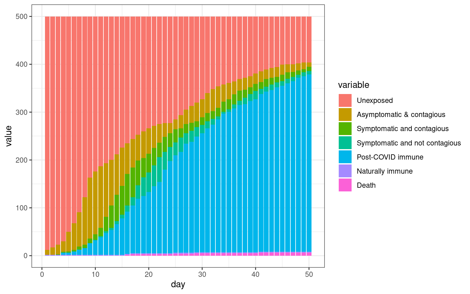
##make the SIR plot:
sir <- data.frame(day=disthist.df$day,
                  susceptible = disthist.df$Unexposed,
                  infected = disthist.df[,2]+disthist.df[,3],
                  recovered = rowSums(disthist.df[,4:7]))

plot4 <- ggplot(melt(sir,id.vars="day"),aes(x=day,group=variable,y=value,color=variable)) + geom_line() + theme_bw() + ggtitle(label="Network simulation with stay at home order from day 10 to 25")
print(plot4)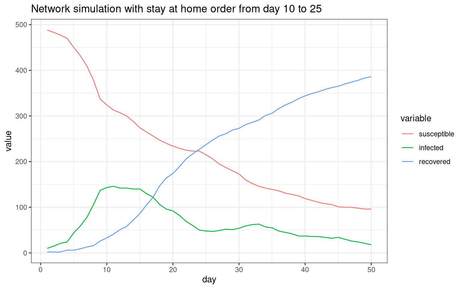
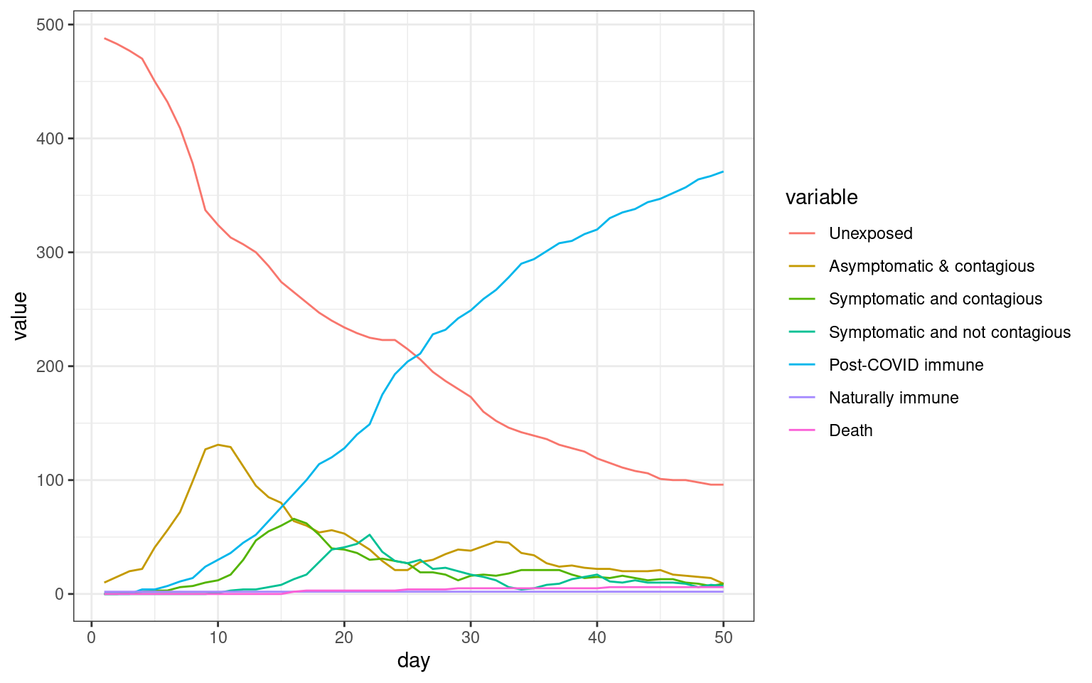
We can see that in this simulation, there were two spikes–one initial one and one that occurred after the stay-at-home order lifted.
Limations of the model
This model allows simulating agent behavior and response at a level not typically incorporated in many of the existing COVID-19 prediction models. It is not a full-fledged model however, and you should not use it for making predictions for your own situations. Whether you should trust the published epidemiological models out there is another issue. What this model permits is easy examination of some of the individual-level behaviors that might impact disease spread, and the impact different policies might have on the outcome.
Summary and other simulations
Feel free to play with the model and try your own simulations. It can help develop understandings of how different psychological, legal, policy, and social aspects can impact the spread of the COVID-19 disease.
There are three student simulations we have developed that help do this, examining how the disease might be impacted by the different demographic networks (schools, workplace, families, etc.), the geography of the state of Michigan, and the possibility of vacationers and travellers bringing the disease into the population.